대표어
대표어


권호기사보기
| 기사명 | 저자명 | 페이지 | 원문 | 기사목차 |
|---|
결과 내 검색
동의어 포함
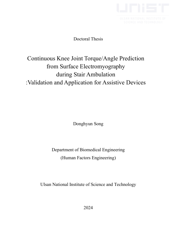
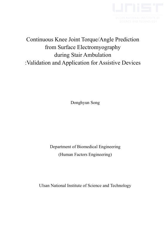
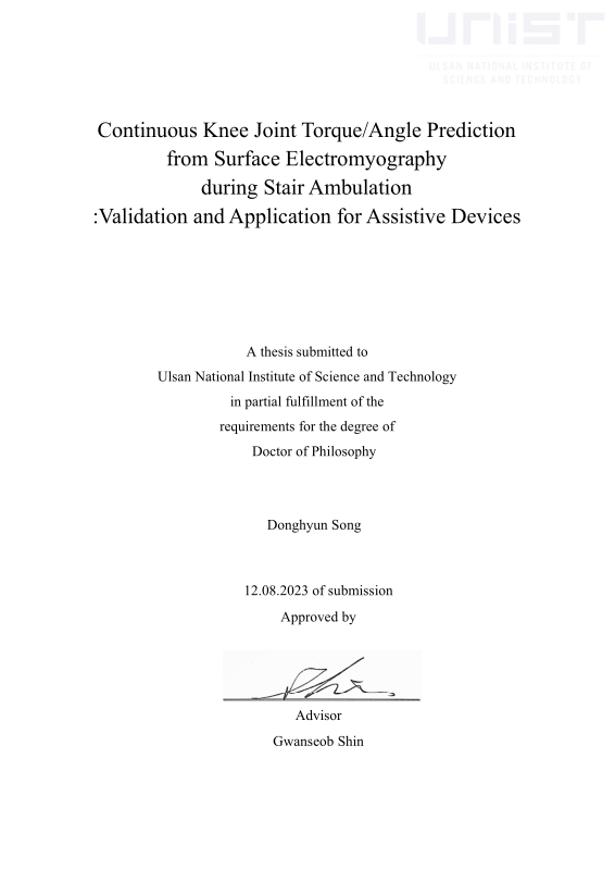
Title Page
ABSTRACT
Contents
EXPLANTION OF TERMS AND ABBREVIATIONS 14
CHAPTER 1. INTRODUCTION 16
1.1. Enhancing Elderly Mobility: Challenges, Innovations, and Prospects 16
1.2. Background 18
1.2.1. History of Lower limb exoskeletons 18
1.2.2. Development of control strategies for lower limb exoskeletons 26
1.2.3. Lower limb exoskeleton control strategy: Using kinematics 27
1.2.4. Lower limb exoskeleton control strategy: Using surface electromyography (sEMG) 35
1.2.5. Application of deep learning in lower limb exoskeleton control 39
1.2.6. Research gap 41
CHAPTER 2. VALIDATION PROCESS 42
2.1. Prediction using nine leg muscles. 42
2.1.1. Objective 42
2.1.2. Methods 42
2.1.3. Results 57
2.1.4. Discussion and Conclusion 59
2.2. Using Five Leg Muscles for Prediction 60
2.2.1. Objective 60
2.2.2. Methods 62
2.2.3. Results 65
2.2.4. Discussion and Conclusion 67
CHAPTER 3. APPLICATION PROCESS 69
3.1. Arising limitation in Chapter 2 69
3.1.1. Are lower limb sEMG signals necessary? 69
3.1.2. Considering various situations is essential. 81
3.1.3. Two objectives of the main experiment 82
3.2. Methods 83
3.3. Results 101
3.3.1. Changes according to the load condition 101
3.3.2. Knee flexion angle prediction 103
3.3.3. Knee joint torque prediction 106
3.4. Discussion and Conclusion 109
CHAPTER 4. CONCLUSION 113
4.1. General conclusion 113
4.2. Future research 115
4.3. Potential application scenario 116
APPENDIX 117
REFERENCES 119
Figure 1.1. Graphical representation of the relationship between age and functional capacity. The graph illustrates the typical trajectory of functional capacity throughout the lifespan,... 16
Figure 1.2. An illustration of a passive lower limb exoskeleton which provides support without electronic components. 19
Figure 1.3. An illustration of an active lower limb exoskeleton equipped with electronic components for enhanced movement assistance. 20
Figure 1.4. The LOKOMAT system, a robotic gait-training device designed for rehabilitative therapy. 22
Figure 1.5. The BLEEX Exoskeleton, designed for enhancing load-carrying endurance of the wearer. 23
Figure 1.6. Ekso™ Exoskeleton, a wearable robotic suit designed to aid individuals with lower-body impairments in walking. 25
Figure 1.7. Trajectory of hip and knee joint angles through a gait cycle, describing the desired trajectory against the measured trajectory. The upper graph presents the hip joint angles, while... 28
Figure 1.8. Illustration of the graph of the reference and the actual knee trajectories of the right knee joint during a real-time experiment with an exoskeleton system. The blue line represents... 29
Figure 1.9. Illustration of the gait cycle phase. 31
Figure 1.10. Right leg joint angles and torque compared to reference during three gait phases for one participant's supported walk. 33
Figure 1.11. Overview of the musculoskeletal modeling framework, detailing the process form data acquisition (A, B) to real time processing and model calibration (C-G), with offline... 37
Figure 2.1. Wireless sEMG and IMU system, Ultium EMG (Image sourced form Noraxon). 44
Figure 2.2. The IMU is placed in the sEMG sensor and its three axes (Retrieved from Noraxon) 44
Figure 2.3. Sensor placement of nine leg muscles. Electrodes were attached to the dominant leg targeting the RF, VL, VM, ST, BF, TA, SL, GM, and GL muscles. These electrodes interfaced... 45
Figure 2.4. Key muscles activated during stair ambulation. The illustration is adapted from the article "Which muscles are used when negotiating stairs?". 45
Figure 2.5. IMU attachment to the participant's dominant leg to record the IMU data. UL: Upper leg; LL: Lower leg 46
Figure 2.6. Specifications of the staircase used in the ambulation task, showing tread depth and riser measurements. 47
Figure 2.7. Illustration of the sEMG sliding window approach in relation to the knee flexion angle. The figure showed the sEMG signals from the vastus lateralis muscle (VL) and the... 50
Figure 2.8. Illustration of the "Leave-one-subject-out" cross-validation method. In each cycle, one subject is assigned for validation (indicated in orange) and another for testing (indicated in... 54
Figure 2.9. Graphical representation of 100ms ahead predictions for knee flexion angle: The blue line showed the predicted knee flexion angle while the red line represents the true knee... 58
Figure 2.10. Graphical representation of 100ms ahead predictions for knee flexion angle: The blue line showed the predicted knee flexion angle while the red line represents the true knee... 58
Figure 2.11. Five sEMG sensor attachment. The electrodes were attached dominant leg at the RF, VL, VM, ST and BF muscle. The electrodes were connected to the sEMG sensors through... 62
Figure 2.12. Graphical representation of 100ms ahead predictions for knee flexion angle: The blue line showed the predicted knee flexion angle while the red line represents the true knee... 66
Figure 2.13. Graphical representation of 100ms ahead predictions for knee flexion angle: The blue line showed the predicted knee flexion angle while the red line represents the true knee... 66
Figure 3.1. Graphical representation of 100ms ahead predictions for knee joint torque: The blue line showed the predicted knee joint torque while the red line represents the true knee joint... 79
Figure 3.2. Sensor placement of five upper leg muscles. Electrodes were attached to the dominant leg targeting the rectus femoris (RF), vastus lateralis (VL), vastus medialis (VM),... 85
Figure 3.3. attachment to the participants dominant leg to record the IMU data. UL: Upper leg; LL: Lower leg. 86
Figure 3.4. Example of additional load used in the experiment, shaped like belts, with evenly distributed additional load: top belt is a 7kg load, and bottom belt is a 5kg load. 88
Figure 3.5. Participant performing stair ambulation tasks under the NA condition: the left figure captures the stair ascending task, and the right figure captures the stair descending task. 90
Figure 3.6. Illustration of the S1 and S2. In each cycle, seven subjects were assigned for training (indicating in black), two subject is assigned for validation (indicated in orange) and another for... 95
Figure 3.7. Illustration of the S3. In each cycle, seven subjects were assigned for training (indicating in black), two subject is assigned for validation (indicated in orange) and another for... 96
Figure 3.8. Illustration of the S4 and S5. In each cycle, seven subjects were assigned for training (indicating in black), two subject is assigned for validation (indicated in orange) and another for... 98
Figure 3.9. Illustration of the S6. In each cycle, seven subjects were assigned for training (indicating in black), two subject is assigned for validation (indicated in orange) and another for... 99
Figure 3.10. Graphical representation of calculated knee joint torque in different additional loading condition: The blue line showed the FA condition, the red line showed the HA condition,... 102
Figure 3.11. Graphical representation of calculated knee joint angle in different additional load condition: The blue line showed the FA condition, the red line showed the HA condition, and the... 102
Figure 3.12. Graphical representation of 100ms ahead predictions for knee flexion angle of S1: The blue line showed the predicted knee flexion angle while the red line represents the true knee... 104
Figure 3.13. Graphical representation of 100ms ahead predictions for knee flexion angle of S2: The blue line showed the predicted knee flexion angle while the red line represents the true knee... 104
Figure 3.14. Graphical representation of 100ms ahead predictions for knee flexion angle of S3: The blue line showed the predicted knee flexion angle while the red line represents the true knee... 105
Figure 3.15. Graphical representation of 100ms ahead predictions for knee joint torque of S4: The blue line showed the predicted knee joint torque while the red line represents the true knee... 107
Figure 3.16. Graphical representation of 100ms ahead predictions for knee joint torque of S5: The blue line showed the predicted knee joint torque while the red line represents the true knee... 107
Figure 3.17. Graphical representation of 100ms ahead predictions for knee joint torque of S6: The blue line showed the predicted knee joint torque while the red line represents the true knee... 108
This study focused on enhancing lower limb exoskeleton functionality for elderly individuals, particularly in navigating the challenges of stair ambulation. The increasing elderly population highlights the need for assistive technologies to support reduced mobility. The research explored control strategies for lower limb exoskeletons, integrating surface electromyography (sEMG) and kinematic data to address limitations in existing control methods. It proposed sEMG-based strategies for assisting elderly stair ambulation.
The research validated an sEMG-based method for predicting knee flexion angles 100ms ahead during stair ambulation by analyzing sEMG signals from leg muscles and testing the accuracy of deep learning models, including 1-D CNN and Vanilla RNN, in predicting future knee angles. It also examined reducing sEMG sensors from nine to five using Vanilla RNN and LSTM models, aiming to simplify the sensor array and enhance user comfort.
Practical applications of these models were tested under various simulated load conditions, reflecting different exoskeleton assistance levels. Bi-LSTM models were used to predict knee flexion angles and joint torques under these conditions. The study's scenarios mimicked varying exoskeleton support levels, assessing model robustness and practicality in real-world exoskeleton usage.
Results showed that the Bi-LSTM models' performance was reasonable in predicting knee flexion angles and less in predicting knee joint torques. However, enhanced predictive performance was observed when applying additional datasets for fine-tuning. Enhanced performance indicated the potential of integrating these models into exoskeleton systems for elderly assistance.
In conclusion, the study showed the significance of these predictive models for developing assistive exoskeletons. Although promising, future research should include a broader participant base, use actual measured values for validation, and implement models in real-time scenarios to improve the practicality and effectiveness of exoskeletons in aiding elderly mobility, especially in complex tasks like stair ambulation.*표시는 필수 입력사항입니다.
| 전화번호 |
|---|
| 기사명 | 저자명 | 페이지 | 원문 | 기사목차 |
|---|
| 번호 | 발행일자 | 권호명 | 제본정보 | 자료실 | 원문 | 신청 페이지 |
|---|
도서위치안내: / 서가번호:
우편복사 목록담기를 완료하였습니다.
*표시는 필수 입력사항입니다.
저장 되었습니다.