대표어
대표어
권호기사보기
| 기사명 | 저자명 | 페이지 | 원문 | 기사목차 |
|---|
결과 내 검색
동의어 포함
목차
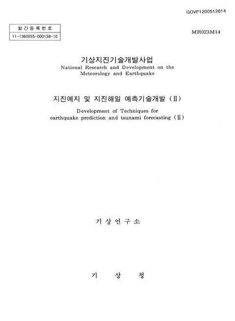
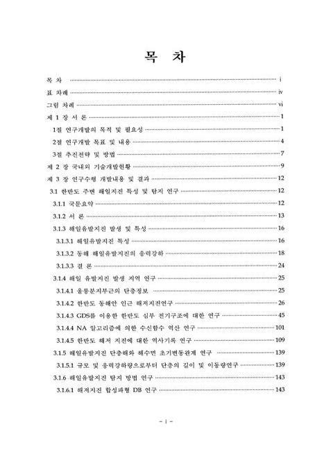
표제지=0,1,1
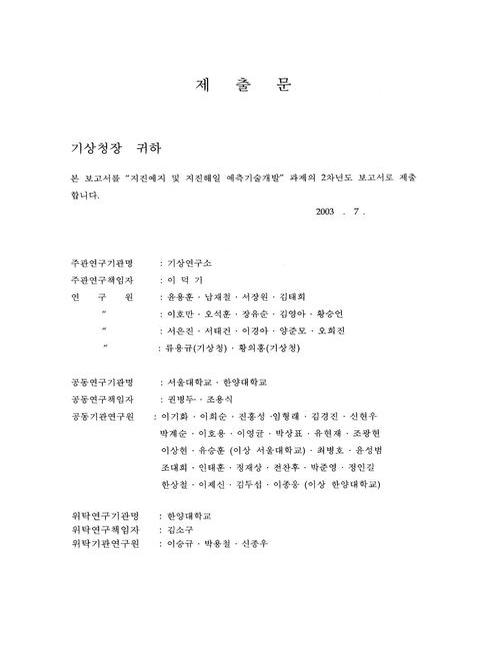
제출문=0,2,1
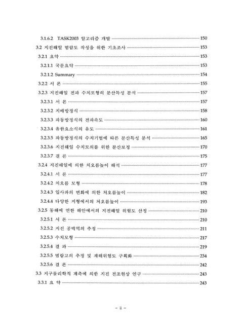
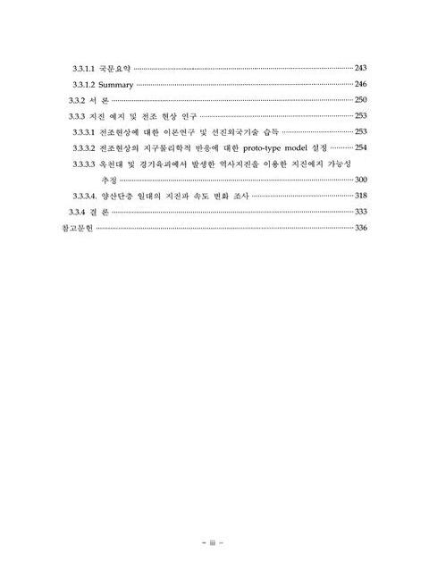
목차=i,3,3
List of Talbe=iv,6,2
List of Figure=vi,8,17
제1장 서론=1,25,1
1절 연구개발의 목적 및 필요성=1,25,3
2절 연구개발 목표 및 내용=4,28,3
3절 추진전략 및 방법=7,31,2
제2장 국내외 기술개발현황=9,33,3
제3장 연구수행 개발내용 및 결과=12,36,1
3.1 한반도 주변 해일지진 특성 및 탐지 연구=12,36,1
3.1.1 국문요약=12,36,1
3.1.2 서론=13,37,3
3.1.3 해일유발지진 발생 및 특성=16,40,1
3.1.3.1 해일유발지진 특성=16,40,3
3.1.3.2 동해 해일유발지진의 응력강하=18,42,7
3.1.3.3 결론=24,48,1
3.1.4 해일 유발지진 발생 지역 연구=25,49,1
3.1.4.1 울릉분지부근의 단층정보=25,49,2
3.1.4.2 한반도 동해안 인근 해저지진연구=26,50,19
3.1.4.3 GDS를 이용한 한반도 심부 전기구조에 대한 연구=45,69,56
3.1.4.4 NA 알고리즘에 의한 수신함수 역산 연구=101,125,8
3.1.4.5 한반도 해저 지진에 대한 역사기록 연구=109,133,30
3.1.5 해일유발지진 단층해와 해수면 초기변동관계 연구=139,163,1
3.1.5.1 규모 및 응력강하량으로부터 단층의 길이 및 이동량연구=139,163,4
3.1.6 해일유발지진 탐지 방법 연구=143,167,1
3.1.6.1 해저지진 합성파형 DB 연구=143,167,8
3.1.6.2 TASK2003 알고리즘 개발=150,174,3
3.2 지진해일 범람도 작성을 위한 기초조사=153,177,1
3.2.1 요약=153,177,1
3.2.1.1 국문요약=153,177,1
3.2.1.2 Summary=154,178,1
3.2.2 서론=155,179,2
3.2.3 지진해일 전파 수치모형이 분산특성 분석=157,181,1
3.2.3.1 서론=157,181,2
3.2.3.2 지배방정식=158,182,3
3.2.3.3 파동방정식의 전파속도=160,184,2
3.2.3.4 유한요소식의 유도=161,185,4
3.2.3.5 파동방정식의 수치기법에 따른 분산특성 분석=165,189,5
3.2.3.6 지진해일 수치모의를 위한 분산보정=170,194,6
3.2.3.7 결론=175,199,2
3.2.4 지진해일에 의한 처오름높이 해석=177,201,1
3.2.4.1 서론=177,201,1
3.2.4.2 처오름 모형=178,202,5
3.2.4.3 입사파의 변화에 의한 처오름높이=182,206,12
3.2.4.4 다양한 지형에서의 처오름높이=193,217,17
3.2.5 동해에 연한 해안에서의 지진해일 위험도 산정=210,234,1
3.2.5.1 서론=210,234,2
3.2.5.2 지진 공백역의 추정=211,235,7
3.2.5.3 수치모형=217,241,2
3.2.5.4 결과=219,243,15
3.2.5.5 범람고의 추정 및 재해위험도 구획화=234,258,8
3.2.5.6 결론=242,266,1
3.3 지구물리학적 계측에 의한 지진 전조현상 연구=243,267,1
3.3.1 요약=243,267,1
3.3.1.1 국문요약=243,267,3
3.3.1.2 Summary=246,270,4
3.3.2 서론=250,274,3
3.3.3 지진 예지 및 전조 현상 연구=253,277,1
3.3.3.1 전조현상에 대한 이론연구 및 선진외국기술 습득=253,277,2
3.3.3.2 전조현상의 지구물리학적 반응에 대한 proto-type model 설정=254,278,46
3.3.3.3 옥천대 및 경기육괴에서 발생한 역사지진을 이용한 지진예지 가능성 추정=300,324,18
3.3.3.4 양산단층 일대의 지진파 속도 변화 조사=318,342,15
3.3.4 결론=333,357,3
참고문헌=336,360,13
Figure 3.1-1. An example of a model for "tsunami earthquake"=17,41,1
Figure 3.1-2. Occurrence of an earthquake due to different rise time (T) with constant moment. a) with shorter rise time (T) and b) with longer rise time=19,43,1
Figure 3.1-3(a). Stress drop as a function of magnitude and fault dimension. Data from Abe (1995) has been used=21,45,1
Figure 3.1-3(b). Stress drop as a function of magnitude and fault dimension. Earthquake data in Donghae has been used=21,45,1
Figure 3.1-4. E/Mo ratio and dip angle as a parameter for tectonic characteristics. Data from Table 3.1-1 has been used=23,47,1
Figure 3.1-5. Fault information around Uleung Basin has been added to the TASK2003=25,49,1
Figure 3.1-6. Instrument response for STS2-Q4128 system based on the poles and zeros on Table 3.1-3=28,52,1
Figure 3.1-7. Epicenter of the earthquake occurred Nov. 24,2001 in 36.7422(이미지참조) and 129.8673(이미지참조)=29,53,1
Figure 3.1-8. Travel time residuals for the earthquake occurred on Nov. 24,2001. a) P travel time residuals using three different velocity models,b) S travel time residuals,and c) P and S residuals are plotted using CUS velocity model=30,54,1
Figure 3.1-9. Waveform fitting after applying Grid Search Technique=31,55,1
Figure 3.1-10. Focal depth obtained from the result of Grid Search Method=32,56,1
Figure 3.1-11. Sensitivity of the result from Grid Search Method. a) each vector is plotted at specific fair of (strike,dip) at an angle of rake degrees (1 degrees is up) with length proportional to the fit value. b) magnified for a)=33,57,1
Figure 3.1-12. The lower hemisphere projection of the focal mechanism with predicted P polarities and amplitude=34,58,1
Figure 3.1-13. Variation on theoretical amplitude due to a) strike variation and b) rake variation at "DAG" station for the earthquake occurred on Nov.,24,2001=35,59,1
Figure 3.1-14. Waveform fitting after applying Grid Search Technique for the event occurred on July,8,2002=36,60,1
Figure 3.1-15. Focal depth obtained from the result of Grid Search Method=37,61,1
Figure 3.1-16. Sensitivity of the result from Grid Search Method for the earthquake occurred on July,8,2002=38,62,1
Figure 3.1-17. a) The lower hemisphere projection of the focal mechanism with predicted P polarities and amplitude for the earthquake occurred on July,8,2002 and b) Epicenter location with fault geometry in the TASK2003=39,63,1
Figure 3.1-18. Inversion results for focal mechanism for the earthquake occurred on Nov.,21,2001. a) synthetic-data match,b) depth sensitivity,c) focal sensitivity,and d) suggested focal mechanism=40,64,1
Figure 3.1-19. Focal mechanism of the earthquakes occurred near the east coast of Korea [a) and b)] and inland [c)]=41,65,1
Figure 3.1-20. Inversion results for focal mechanism for the earthquake occurred on June,15,2000=42,66,1
Figure 3.1-21. Synthetics of the earthquake occurred on May 26,1983 at 40.65(이미지참조) and 139.03(이미지참조)=43,67,1
Figure 3.1-22. Synthetics on "DAG" station. Only Pn and Sn Part have been plotted=44,68,1
Figure 3.1-23. The three-components of geomagnetic field that observed at Icheon and the power spectrum for the time variations of the magnetic field. (a),(b) and (c) denote northern,eastern and vertical magnetic field components,respectively.=49,73,1
Figure 3.1-24. Kasier-Bessel window for alpha=50,74,1
Figure 3.1-25. Example of Huber's M-estimator(Hber,1982). The discontinuous point is (이미지참조),(이미지참조)=57,81,1
Figure 3.1-26. Q-Q(Quantile-quantile) plots at the Icheon observatory. They show tailed residual distributions for long periods due to source effect and short periods due to local environmental noises=60,84,1
Figure 3.1-27. Induction length and phase of geomagnetic transfer function at Icheon observatory(after Parkinson's convention). The star(☆) and the triangle(▲) denote conventional least square estimation,robust estimation,respectively=61,85,1
Figure 3.1-28. Q-Q(Quantile-quantile) plots at the Yongin observatory. They show tailed residual distributions for short periods due to local environmental noises=62,86,1
Figure 3.1-29. Induction length and phase of geomagnetic transfer function at Yongin observatory(after Parkinson's convention). The star(☆) and the triangle(▲) denote conventional least square estimation,robust estimation,respectively=63,87,1
Figure 3.1-30. The two-dimensional numerical models for (S) sea-land model (C) conductor-land model (SC) sea-land-conductor model=69,93,1
Figure 3.1-31. The responses at six periods of variations of the sea-land model(S). A horizontal scale in above graph is 200km=70,94,1
Figure 3.1-32. The responses at six periods of variations of the conductor-land (C) model. A horizontal scale in above graph is 200km=71,95,1
Figure 3.1-33. The responses at six periods of variations of the sea-land-conductor model(SC,Model 1). It shows the SC(solid line) response and the algebraic summed response S+C(circle),respectively. The distance between sea and conductor is 40km and...=72,96,1
Figure 3.1-34. The two-dimensional numerical model to examine the validity of difference arrow with respect to distance between sea and conductor. The distances between them are 120km(Model 2) and 200km(Model 3),respectively=74,98,1
Figure 3.1-35. The responses at six periods of variations of the Model 2. It shows the SC(solid line) response and the algebraic summed response S+C(circle). The distance between sea and conductor is 120km and a horizontal scale in above graph is 200km=75,99,1
Figure 3.1-36. The results are the same as in Fig. 6 except distance of 200km between sea and conductor=76,100,1
Figure 3.1-37. The two-dimensional numerical model to examine the validity if difference arrow with respect to the buried depth(Model 4) and the size(Model 5) of the conductor. The horizontal distance between sea and conductor is 120 km same...=78,102,1
Figure 3.1-38. The responses at six periods of variation of the Model 4. It shows the SC response(solid line) and the algebraic summed response S+C(circle). The buried depth of the conductor is 28km and a horizontal scale in above graph is 200km=79,103,1
Figure 3.1-39. The responses at six periods of variation of the Model 5. It shows the SC response(solid line) and the algebraic summed response S+C(circle). The vertical extension of the conductor is up to 31km and a horizontal scale in above graph...=80,104,1
Figure 3.1-40. 3-D image of the numerical model. The 2-D extensions expand x,y directions and 1-D extension expands z direction,respectively. The plan view shows x-y and x-z section of the numerical model=83,107,1
Figure 3.1-41. The three-dimensional numerical model sea-land model(S),conductor-land model(C),and sea-land-conductor model(SC),respectively=86,110,1
Figure 3.1-42. Real and imaginary induction vectors for (a) Sea-only model,(b) Conductor-only model,and (c) Sea-conductor model. The period of field is 40 min. The scale of x and y axis means the grid number in the numerical model=87,111,1
Figure 3.1-43. Real and imaginary induction vectors for (a) Sea-only model,(b) Conductor-only model,and (c) Sea-conductor model. The period of field is 10 min. The scale of x and y axis means the grid number in the numerical model=88,112,1
Figure 3.1-44. Vectors ◁(이미지참조) for SC(=89,113,1
Figure 3.1-45. The three-dimensional numerical model to examine the validity of difference arrow according to distance between sea and conductor. The distance between them is 30 km (Model 1),90 km (Model 2),and 150 km (Model 3),respectively=91,115,1
Figure 3.1-46. Vectors ◁(이미지참조) for the three positions of conductor shown in Figure 3.1-28. (a) Model 1,(b) Model 2,(c) Model 3,respectively. The period of field is 10 min=92,116,1
Figure 3.1-47. The three-dimensional numerical model to examine the validity of difference arrow according to the buried depth (Model 4) and the size (Model 5) of the conductor. The horizontal distance between sea and conductor is 90 km as in the...=94,118,1
Figure 3.1-48. Vectors ◁(이미지참조) for (a)Model 2,(b)Model 4,respectively. The period of field is 10 min=95,119,1
Figure 3.1-49. Vectors ◁(이미지참조) for (a)Model 4,(b)Model 5,respectively. The period of field is 10 min=96,120,1
Figure 3.1-50. The three-dimensional numerical model to examine the validity of difference arrow for conductor which is vertically extended down to the deep part. The horizontal distance between sea and conductor is 90 km as in the case...=97,121,1
Figure 3.1-51. Vectors ◁(이미지참조) for (a)Model 2,(b)Model 6,respectively. The period of field is 40 min=98,122,1
Figure 3.1-52. Vectors ◁(이미지참조) for (a)Model 2,(b)Model 6,respectively. The period of field is 10 min=99,123,1
Figure 3.1-53. Random points and their Voronoi cells=103,127,1
Figure 3.1-54. Model density plot for models produced by the neighborhood algorithm. The best data-fitting model is plotted in red,and the true model is in cyan. The color scale shows the increase in data-fit,from yellow to green. The outline...=105,129,1
Figure 3.1-55. Receiver functions of the true (black) and best fit (blue)=106,130,1
Figure 3.1-56. Ensembles produced by NA projected onto tow pairs of parameter axis (labelled). The best of the 10,000 models in each panel is believed to be in the middle of the red points and the true model is appeared as a blue +. The dots are...=107,131,1
Figure 3.1-57. Isoseismal map for the Ms 7.3 Haeseong earthquake occurred on Feb. 4,1975,(Modified from Oh(1996))=111,135,1
Figure 3.1-58. Isoseismal map of Korea for the Ms 7.3 Haeseong earthquake occurred on Feb. 4,1975=122,146,1
Figure 3.1-59. Isoseismal map for the earthquake occurred near the offshore of Ulsan on July 24,1643=129,153,1
Figure 3.1-60. Isoseismal map for the earthquake occurred near the offshore of Cheongam-sa,Buryung-bu,Hamkyung province on Feb. 19,1810=137,161,1
Figure 3.1-61. Velocity models used for making Green's Function using Reflectivity method=146,170,1
Figure 3.1-62. An example of synthetic-data match using DB for the earthquake occurred on June,15,2000 near the Southeastern part of Japan close to the Trench=147,171,1
Figure 3.1-63. An example of synthetic-data match from body wave to surface wave using DB for the earthquake occurred on June,15,2000 near the Southeastern part of Japan close to the Trench. Station name and components are written in the Top and...=148,172,1
Figure 3.1-64. Magnification of "TAG" radial component shown in the Figure 3.1-63=149,173,1
Figure 3.1-65. Main-window of TASK2003 for finding fault information and calculating tsunami information based on that fault information=151,175,1
Figure 3.1-66. Fault information based on the given epicenter location(cross-hair) is given in the left part of figure=151,175,1
Figure 3.1-67. Calculated theoretical traveltimes and waveforms of the tsunami near the east coast of the major points of Korea=152,176,1
Figure 3.2-1. Relative phase error of wave equation=162,186,1
Figure 3.2-2. Coordinate system and initial free surface profile to test the accuracy of numerical scheme=168,192,1
Figure 3.2-3. Free surface profiles at t=169,193,1
Figure 3.2-4. Initial free surface profile of Gaussian hump=172,196,1
Figure 3.2-5. Schematic sketch to calculate analytical solution=172,196,1
Figure 3.2-6. Comparison of free surface profiles at t=173,197,1
Figure 3.2-7. Comparison of free surface profiles at t=173,197,1
Figure 3.2-8. Comparison of free surface profiles at t=175,199,1
Figure 3.2-9. A schematic sketch of moving boundary treatment(Yoon and Cho,2001)=181,205,1
Figure 3.2-10. Top view of the wave basin and the island and vertical view of the circular island=183,207,1
Figure 3.2-11. Snapshot of free surface displacements=184,208,1
Figure 3.2-12. Snapshot of velocity distribution in the vicinity of the circular island=185,209,1
Figure 3.2-13. Comparison of maximum run-up height around the circular island=186,210,1
Figure 3.2-14. Instantaneous shoreline locations in front of the island for (이미지참조)=186,210,1
Figure 3.2-15. Instantaneous shoreline locations in the lee of the island for (이미지참조)=187,211,1
Figure 3.2-16. Comparison of maximum run-up height around the circular island;(이미지참조)-0.1,(이미지참조)=189,213,1
Figure 3.2-17. Comparison of maximum run-up height around the circular island;(이미지참조)=190,214,1
Figure 3.2-18. Comparison of maximum run-up height around the circular island;(이미지참조)=191,215,1
Figure 3.2-19. Comparison of maximum run-up height around the circular island;(이미지참조)=191,215,1
Figure 3.2-20. Comparison of maximum run-up height around the circular island;(이미지참조)=192,216,1
Figure 3.2-21. Comparison of maximum run-up height around the circular island;(이미지참조)=193,217,1
Figure 3.2-22. Comparisons of the normalized runup height distribution around the circular and elliptic islands;(이미지참조)=195,219,1
Figure 3.2-23. (a) Top view of the wave basin and the island. (b) Vertical view of the circular island on the cross-section C-C=198,222,1
Figure 3.2-24. Snapshot of free surface displacements=199,223,1
Figure 3.2-25. Snapshots of velocity distribution at different times=200,224,1
Figure 3.2-26. Snapshots of velocity distribution at different times=201,225,1
Figure 3.2-27. Free surface configurations in the lee of the islands at t=202,226,1
Figure 3.2-28. Free surface configurations in front of the islands;(이미지참조)=202,226,1
Figure 3.2-29. Instantaneous shoreline locations in front of the island for (이미지참조)/D=203,227,1
Figure 3.2-30. Instantaneous shoreline locations in front of the island for (이미지참조)/D=203,227,1
Figure 3.2-31. Maximum runup heights on the inside and outside of the island=205,229,1
Figure 3.2-32. Maximum runup heights on the inside of two island=206,230,1
Figure 3.2-33. Maximum runup heights on the outside of two island=207,231,1
Figure 3.2-34. Maximum runup heights on the inside of two island=208,232,1
Figure 3.2-35. Maximum runup heights on the outside of two island=209,233,1
Figure 3.2-36. Bathymetry of the East Sea=212,236,1
Figure 3.2-37. Seismic gap(Ichikawa,1994)=213,237,1
Figure 3.2-38. Faults parameters=214,238,1
Figure 3.2-39. The location of hypothetical tsunamigenic earthquakes with fault models of detailed parameters(left) and simple shape sources(right)=215,239,1
Figure 3.2-40. Initial elevation of hypothetical tsunamigenic earthquakes with fault models of detailed parameters=216,240,1
Figure 3.2-41. Initial elevation of simple shape sources=217,241,1
Figure 3.2-42. Geographical locations of coasts adjacent to the East Sea divided by five regions=221,245,1
Figure 3.2-43. Spatial distribution of the wave heights showing geographical zones with low risk of tsunami as arrows(left columned diagrams are based on hypothetical tsunamigenic earthquakes with fault models of detailed parameters and right...=222,246,1
Figure 3.2-44. The same normalized on maximum showing geographical zones with low risk of tsunami as arrows(left columned diagrams are based on hypothetical tsunamigenic earthquakes with fault models of detailed parameters and right column are...=223,247,1
Figure 3.2-45. Relation between max and mean values of the wave heights at different locations based on hypothetical tsunamigenic earthquakes with fault models of detailed parameters=227,253,1
Figure 3.2-46. Relation between max and mean values of the wave heights at different locations based on tsunamis by simple shape initial elevation=229,255,1
Figure 3.2-47. Specific positions that are estimated Hprog and observed runup heights of 1983(a) and 1993(b) tsunamis on the East Coast in Korea=235,259,1
Figure 3.2-48. Specific positions that are estimated Hprog and observed runup heights of 1983(a) and 1993(b) tsunamis in Primorskii=236,260,1
Figure 3.2-49. Specific positions that are estimated Hprog and observed runup heights of 1983(a) and 1993(b) tsunamis in Sakhalin I. and Hokkaido=237,261,1
Figure 3.2-50. Specific positions that are estimated Hprog and observed runup heights of 1983(a) and 1993(b) tsunamis in Sakhalin I. and Honshu=238,262,1
Figure 3.2-51. Tsunami risk zonation for coasts adjacent regions to the East Sea(used by tsunamis by an earthquake with detailed faults parameters and simple shape initial elevation)=241,265,1
Figure 3.2-52. Tsunami risk zonation for coasts adjacent regions to the East Sea(left columned map is for tsunamis by an earthquake with detailed faults parameters and right columned one is for tsunamis by simple shape initial elevation)=241,265,1
Figure 3.3-1. Real-Time Fault Monitoring areas=253,277,1
Figure 3.3-2. MT response at TM mode for a fault model with shallow heterogeneity=255,279,1
Figure 3.3-3. Geology map of Hongsung area=263,287,1
Figure 3.3-4. Location map with sites of AMT survey(triangle) and a line of DC resistivity survey(arrow line)=263,287,1
Figure 3.3-5. Array configuration of DC resistivity and AMT survey on the central region. The fault line lies in Y direction=264,288,1
Figure 3.3-6. Results of DC resistivity survey=264,288,1
Figure 3.3-7. Pseudosections of AMT survey:(a) TM mode and (b) TE mode=265,289,1
Figure 3.3-8. 1-D MT inversion result of HS_11 site using Marquardt-Levenberg method. Initial values are applied from the decimated model of Bostick inversion results=265,289,1
Figure 3.3-9. 2-D MT inversion results using (a) rapid relaxation inversion and (b)non-linear conjugate gradient algorithm=266,290,1
Figure 3.3-10. Comparison between DC resistivity survey and AMT survey. Upper section is the resistivity section of DC survey and lower section is the section of MT inversion using non-linear conjugate gradient inversion. Solid lines are left and...=267,291,1
Figure 3.3-11. Schematic behavior of the modulated electromagnetic field by the conductivity fluctuation in the case of (a) (이미지참조) ≪ (이미지참조) and (b) (이미지참조) ≫ (이미지참조),where (이미지참조) and (이미지참조) are the frequencies of...=277,301,1
Figure 3.3-12. Section view of two-dimensional model which includes a conductive fault zone=278,302,1
Figure 3.3-13. (a) Background magnetic fields (H(이미지참조)) at the four frequencies. (b) Anomalous (modulated) magnetic fields due to modulation of each low frequency electromagnetic field in the case that the frequency of conductivity fluctuation...=279,303,1
Figure 3.3-14. The shape of (a) modulated magnetic field and (b) modulated magnetic field normalized with the ratio of one-dimensional impedance=280,304,1
Figure 3.3-15. (a) Power spectra of natural magnetic field and derived electric field at the Ichon geomagnetic observatory. The power spectrum of electric field is derived from magnetic field spectrum using the impedance for the one-dimensional model.=281,305,1
Figure 3.3-16. Amplitude ratio between modulated and normal magnetic field. The amplitude and frequency of conductivity fluctuation are 0.1 and 0.1Hz,respectively. The amplitude of normal magnetic field is calculated in a narrow frequency band...=282,306,1
Figure 3.3-17. Amplitude ratio between modulated and normal magnetic field according to the frequency of conductivity fluctuation:0.1 Hz,0.03 Hz and 0.01 Hz=283,307,1
Figure 3.3-18. Amplitude ratio between modulated and normal magnetic field according to the conductivity of fault zone:3 Ohm-m,30 Ohm-m and 300 Ohm-m=283,307,1
Figure 3.3-19. Comparison of the responses according to the different one-dimensional crustal structures. (a) one-dimensional crustal structure of model A. (b) one-dimensional crustal structure of model B with more conductive layers. (c) variances of...=284,308,1
Figure 3.3-20. Predicted changes during earthquake cycle for dilatancy model(Scholz,1973)=287,311,1
Figure 3.3-21. Two vertical layers showing the effects of variation of the resistivity and permeability=296,320,1
Figure 3.3-22. Two Inclined layers showing the effects of variation of the resistivity and permeability=297,321,1
Figure 3.3-23. Self-potential variation at San Andreas fault zone at December 1975(Corwin,1977)=298,322,1
Figure 3.3-24. Differential magnetic field at occurrence of earthquake=299,323,1
Figure 3.3-25. The cumulative earthquake data occurred in Okcheon Belt and Kyeonggi Massif,and the derived frequency-intensity relation of the earthquakes=308,332,1
Figure 3.3-26. The cumulative earthquake data of foreshocks,main shock and aftershocks (a),and just foreshocks of the earthquake occurred on March 9,1437 and derived each frequency-intensity relations=309,333,1
Figure 3.3-27. The cumulative earthquake data of foreshocks,main shock and aftershocks (a),and just foreshocks of the earthquake occurred on October 17,1531 and derived each frequency-intensity relations=310,334,1
Figure 3.3-28. The cumulative earthquake data of foreshocks,main shock and aftershocks (a),and just foreshocks of the earthquake occurred on December 31,1557 and derived each frequency-intensity relations=311,335,1
Figure 3.3-29. The cumulative earthquake data of foreshocks,main shock and aftershocks (a),and just foreshocks of the earthquake occurred on March 19,1682 and derived each frequency-intensity relations=312,336,1
Figure 3.3-30. The cumulative earthquake data of foreshocks,main shock and aftershocks (a),and just foreshocks of the earthquake occurred on July 30,1757 and derived each frequency-intensity relations=313,337,1
Figure 3.3-31. The cumulative earthquake data of foreshocks,main shocks and aftershocks (a),and the just foreshocks (b) of the summed earthquakes and derived each frequency-intensity relation=314,338,1
Figure 3.3-32. The diagram shows the regression plot of b and Dc in Kyunggi Massif. A negative correlation between b and Dc was implied=315,339,1
Figure 3.3-33. The diagram shows the regression plot of b and Dc in Okcheon zone. A negative correlation between b and Dc was implied=316,340,1
Figure 3.3-34. The diagram shows the regression plot of b and Dc in Kyungsang Basin. A negative correlation between b and Dc was implied=317,341,1
Figure 3.3-35. Schematic diagram of two station method=326,350,1
Figure 3.3-36. Location map of the earthquake events used in this study and the short period KIGAM seismic stations. Open circle represents assumed dilatancy area of chosen earthquakes in 1999 listed in the Table 3.3-3 (Number 2,3,and 5).=326,350,1
Figure 3.3-37. Time picking of the first P and S-wave motions. Three-component waveforms of the 18 September 1998 earthquake recorded at the station KMH of KIGAM seismograph network. The local magnitude of the earthquake is 2.5 and epicentral distance...=327,351,1
Figure 3.3-38. The seismic ray paths between KIGAM short period stations in Yang-San area and events which have ray paths through assumed dilatancy area of chosen earthquakes listed in Table 3.3-3 (Number 2,3,and 5). Cross marks,triangles and circle...=328,352,1
Figure 3.3-39. Travel time curve for the primary waves in the Choi (2002)'s crustal model. Note that direct wave is arrived first to about 120km=329,353,1
Figure 3.3-40. Temporal variations of the values of Vp/Vs ((이미지참조)) near the chosen area. The origin times of earthquakes of mid-size (over 2.5) magnitude occurred in the Yang-san area are shown along the time axis by arrows. The information...=329,353,1
Figure 3.3-41. Temporal variation of the values of apparent P-wave and S-wave velocity near the chosen area. The origin times of earthquakes of mid-size (over 2.5) magnitude occurred in the Yang-San area are shown along the time axis by arrows.=330,354,1
Figure 3.3-42. Temporal variation of the values of P-wave travel time residual calculated using Choi(2002)'s crustal model. RMS error is 0.44. The dashed line indicates zero residual. The origin times of earthquakes of mid-size (over 2.5) magnitude...=330,354,1
Figure 3.3-43. Temporal variation of the values of Vp/Vs ((이미지참조)),apparent P-wave and S-wave velocity and P-wave travel time residual near the chosen area. The dashed lines indicate normal value (1.75) of Vp/Vs ((이미지참조)) in Poisson...=331,355,1
Figure 3.3-44. Locations of assumed dilatancy area of a earthquake occurred on 12 September 1999(5),19 May 2000(13),and 23 September 2000(15) and two earthquakes (cross mark,A and B) used in calculating two abnormal Vp/Vs ((이미지참조)). The solid...=332,356,1
jpg
Figure 3.1-8. Travel time residuals for the earthquake occurred on Nov. 24,2001. a) P travel time residuals using three different velocity models,b) S travel time residuals,and c) P and S residuals are plotted using CUS velocity model=30,54,1
Figure 3.1-11. Sensitivity of the result from Grid Search Method. a) each vector is plotted at specific fair of (strike,dip) at an angle of rake degrees (1 degrees is up) with length proportional to the fit value. b) magnified for a)=33,57,1
Figure 3.1-13. Variation on theoretical amplitude due to a) strike variation and b) rake variation at "DAG" station for the earthquake occurred on Nov.,24,2001=35,59,1
Figure 3.1-16. Sensitivity of the result from Grid Search Method for the earthquake occurred on July,8,2002=38,62,1
Figure 3.1-17. a) The lower hemisphere projection of the focal mechanism with predicted P polarities and amplitude for the earthquake occurred on July,8,2002 and b) Epicenter location with fault geometry in the TASK2003=39,63,1
Figure 3.1-18. Inversion results for focal mechanism for the earthquake occurred on Nov.,21,2001. a) synthetic-data match,b) depth sensitivity,c) focal sensitivity,and d) suggested focal mechanism=40,64,1
Figure 3.1-19. Focal mechanism of the earthquakes occurred near the east coast of Korea [a) and b)] and inland [c)]=41,65,1
Figure 3.1-24. Kasier-Bessel window for alpha=50,74,1
Figure 3.1-54. Model density plot for models produced by the neighborhood algorithm. The best data-fitting model is plotted in red,and the true model is in cyan. The color scale shows the increase in data-fit,from yellow to green. The outline...=105,129,1
Figure 3.1-56. Ensembles produced by NA projected onto tow pairs of parameter axis (labelled). The best of the 10,000 models in each panel is believed to be in the middle of the red points and the true model is appeared as a blue +. The dots are...=107,131,1
Figure 3.1-60. Isoseismal map for the earthquake occurred near the offshore of Cheongam-sa,Buryung-bu,Hamkyung province on Feb. 19,1810=137,161,1
Figure 3.1-65. Main-window of TASK2003 for finding fault information and calculating tsunami information based on that fault information=151,175,1
Figure 3.1-66. Fault information based on the given epicenter location(cross-hair) is given in the left part of figure=151,175,1
Figure 3.2-25. Snapshots of velocity distribution at different times=200,224,1
Figure 3.2-26. Snapshots of velocity distribution at different times=201,225,1
Figure 3.2-27. Free surface configurations in the lee of the islands at t=202,226,1
Figure 3.2-28. Free surface configurations in front of the islands;λ=36m=202,226,1
Figure 3.3-2. MT response at TM mode for a fault model with shallow heterogeneity=255,279,1
Figure 3.3-14. The shape of (a) modulated magnetic field and (b) modulated magnetic field normalized with the ratio of one-dimensional impedance=280,304,1
Figure 3.3-21. Two vertical layers showing the effects of variation of the resistivity and permeability=296,320,1
Figure 3.3-22. Two Inclined layers showing the effects of variation of the resistivity and permeability=297,321,1
Figure 3.3-24. Differential magnetic field at occurrence of earthquake=299,323,1
Figure 3.3-35. Schematic diagram of two station method=326,350,1
Figure 3.3-36. Location map of the earthquake events used in this study and the short period KIGAM seismic stations. Open circle represents assumed dilatancy area of chosen earthquakes in 1999 listed in the Table 3.3-3 (Number 2,3,and 5).=326,350,1
Figure 3.3-39. Travel time curve for the primary waves in the Choi (2002)'s crustal model. Note that direct wave is arrived first to about 120km=329,353,1
Figure 3.3-40. Temporal variations of the values of Vp/Vs ((이미지참조)) near the chosen area. The origin times of earthquakes of mid-size (over 2.5) magnitude occurred in the Yang-san area are shown along the time axis by arrows. The information...=329,353,1
Figure 3.3-41. Temporal variation of the values of apparent P-wave and S-wave velocity near the chosen area. The origin times of earthquakes of mid-size (over 2.5) magnitude occurred in the Yang-San area are shown along the time axis by arrows.=330,354,1
Figure 3.3-42. Temporal variation of the values of P-wave travel time residual calculated using Choi(2002)'s crustal model. RMS error is 0.44. The dashed line indicates zero residual. The origin times of earthquakes of mid-size (over 2.5) magnitude...=330,354,1
Figure 3.3-43. Temporal variation of the values of Vp/Vs ((이미지참조)),apparent P-wave and S-wave velocity and P-wave travel time residual near the chosen area. The dashed lines indicate normal value (1.75) of Vp/Vs ((이미지참조)) in Poisson...=331,355,1
Figure 3.3-44. Locations of assumed dilatancy area of a earthquake occurred on 12 September 1999(5),19 May 2000(13),and 23 September 2000(15) and two earthquakes (cross mark,A and B) used in calculating two abnormal Vp/Vs ((이미지참조)). The solid...=332,356,1
*표시는 필수 입력사항입니다.
| 전화번호 |
|---|
| 기사명 | 저자명 | 페이지 | 원문 | 기사목차 |
|---|
| 번호 | 발행일자 | 권호명 | 제본정보 | 자료실 | 원문 | 신청 페이지 |
|---|
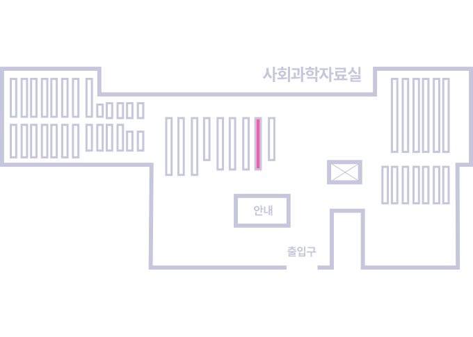
도서위치안내: / 서가번호:
우편복사 목록담기를 완료하였습니다.
*표시는 필수 입력사항입니다.
저장 되었습니다.