대표어
대표어
권호기사보기
| 기사명 | 저자명 | 페이지 | 원문 | 기사목차 |
|---|
결과 내 검색
동의어 포함
목차
표제지=0,1,1
제출문=0,2,1
요약문=3,3,10
SUMMARY=13,13,10
목차=23,23,6
CONTENTS=29,29,8
그림목차(List of Figures)=37,37,20
표목차(List of Tables)=57,57,6
제1장 서론=63,63,3
제1절 연구의 배경 및 필요성=65,65,3
제2절 연구개발목표 및 연구내용=68,68,3
제2장 국내외 기술개발 현황=71,71,3
제1절 서론=73,73,2
제2절 국외 기술개발 현황=74,74,1
1. 미국=74,74,1
가. 연구동향=74,74,2
나. 습지복원ㆍ창출을 위한 표준지침=75,75,5
다. 인공습지 조성기법=79,79,2
라. 인공습지 침식방지 구조물=80,80,1
2. 일본=80,80,1
가. 연구동향=80,80,2
나. 인공갯벌 조성단계별 고려사항=81,81,4
다. 조성사례=84,84,2
3. 유럽=85,85,1
가. 연구동향=85,85,4
나. 조성사례=88,88,3
제3절 국내 기술개발 현황=90,90,1
1. 방조제 축조에 따른 퇴적환경변화=90,90,1
가. 강화지구=90,90,5
나. 대호지구=94,94,2
다. 새만금지구=95,95,2
2. 인공습지 조성사례=96,96,2
3. 연안개발에 따른 저서생태환경 변화=97,97,1
가. 태안화력 발전소 건설사업 환경영향평가서(1988)=97,97,2
나. 태안화력발전소 건설에 따른 피해영향범위조사와 피해어업권 및 어선손실보상액 산출(1995)=98,98,1
다. 태안화력발전소 주변 해양생태계 및 해양환경조사(1998)=98,98,2
라. 태안화력발전소 주변 해양생태계 및 해양환경조사 결과(2000)=99,99,1
마. 주변 해양생태계 및 환경영향조사 결과의 비교=99,99,1
4. 수리ㆍ퇴적현상 관측기술 및 퇴적물 이동 제어기술=99,99,2
가. 수리ㆍ퇴적현상 관측기술=100,100,3
나. 퇴적물이동 제어시설=102,102,1
제3장 연구개발수행 내용 및 결과 I:현장관측ㆍ분석 및 파랑변형 수치실험=103,103,3
제1절 서론=105,105,1
제2절 해수 및 퇴적물의 화학적 특성=106,106,1
1. 서론=106,106,1
2. 조사 및 분석방법=106,106,1
가. 시료채취 및 보존방법=106,106,3
나. 분석방법=109,109,2
3. 결과 및 고찰=110,110,1
가. 해수=110,110,10
나. 퇴적물=119,119,17
다. 갯벌의 정화능력=135,135,4
4. 결론=139,139,1
제3절 연안 저서생태=140,140,1
1. 서론=140,140,1
2. 조사 및 분석 방법=140,140,1
가. 시료채집=140,140,6
나. 표서동물상 조사=145,145,1
다. 분석방법=145,145,2
3. 결과 및 고찰=146,146,1
가. 대형저서생물=146,146,50
나. 중형저서생물=196,196,25
4. 결론=221,221,5
제4절 해저지형 및 퇴적물 특성변화=226,226,1
1. 서론=226,226,1
2. 현장조사 및 분석 방법=227,227,1
가. 해저지형=227,227,1
나. 조간대 퇴적단면고=227,227,3
다. 해저퇴적물=229,229,6
3. 결과 및 고찰=234,234,1
가. 해저지형=234,234,1
나. 조간대 퇴적단면고의 변화=234,234,15
다. 해저퇴적물분포=248,248,1
라. 조간대 퇴적물특성의 변화=248,248,27
4. 요약=274,274,2
제5절 조간대의 퇴적역학 및 침식/퇴적 변화 특성=276,276,1
1. 서론=276,276,3
2. 조사 및 분석 방법=279,279,1
가. 표층퇴적물 채취 및 분석 방법=279,279,1
나. 조간대 퇴적역학 및 침식/퇴적 변화 관측=279,279,3
3. 결과 및 고찰=282,282,1
가. 조사측선의 표층퇴적물 특성=282,282,9
나. 조석/조류 및 파랑의 시계열 분포=291,291,22
다. 조간대 부유퇴적물의 거동=313,313,9
라. 조간대 해저면의 지형(침식/퇴적) 변화=321,321,4
마. 조간대 퇴적물 이동=325,325,16
4. 결론=341,341,2
제6절 탄성파탐사=343,343,1
1. 서론=343,343,1
2. 다중채널 탄성파탐사=343,343,1
가. 자료획득=343,343,4
나. 자료처리=347,347,5
3. 천부지층 탐사 및 Vibro-coring=351,351,7
4. 자료해석=358,358,3
5. 결론=360,360,1
제7절 조석ㆍ조류=361,361,1
1. 개요=361,361,1
2. 현장관측 및 분석=361,361,1
가. 조석=361,361,3
나. 조류=363,363,12
제8절 파랑=375,375,1
1. 개요=375,375,2
2. 자료분석 방법=377,377,2
3. 단주기파 현장관측 및 분석 결과=379,379,1
가. 정점 W1과 W2(파향ㆍ파고계)=379,379,11
나. 정점 P1=389,389,3
다. 정점 P2=392,392,1
라. 정점 P3=392,392,10
마. 정점 P4=401,401,11
바. 천해역에서의 전파ㆍ변형=412,412,1
사. 장안퇴 전후의 파랑 변형=412,412,8
아. 파고간의 상관관계 검토=419,419,9
4. 토의=427,427,1
제9절 파랑변형 수치실험=428,428,1
1. 수치모형 수립=428,428,1
가. 기본방정식=428,428,2
나. 방향 스펙트럼의 설정=429,429,2
다. 유의파 제원 및 파향의 계산=430,430,1
라. 천수변형 과 굴절계수의 계산=430,430,2
2. 파랑의 천해역 변형 수치실험=431,431,1
가. 입력자료 준비=431,431,1
나. 파랑의 천해역 전파ㆍ변형 특성=431,431,9
다. 토의=439,439,2
제10절 조하대 및 퇴적촉진시설 전ㆍ후 퇴적물 거동 종합관측=441,441,2
1. 추계 관측결과=443,443,6
2. 동계 관측결과=448,448,19
3. 결론 및 토의=466,466,3
제4장 연구개발 수행내용 및 결과 II:퇴적촉진시설 설치 및 사후모니터링=469,469,3
제1절 서론=471,471,2
제2절 퇴적촉진 시설물 추가 설치 및 보수=472,472,1
1. 개요=472,472,1
2. 목재 잠제형 퇴적촉진시설의 설계,제작,설치 및 보수=472,472,4
제3절 퇴적물 분포특성=476,476,1
1. 서론=476,476,1
2. 현장조사 및 분석방법=476,476,4
3. 결과 및 고찰=479,479,1
가. S-정점의 퇴적물 조성 및 조직변수=479,479,5
나. 격월간 표층퇴적물의 조직변수 및 퇴적상 변화=483,483,3
다. 캔코어 퇴적물=485,485,20
4. 요약=505,505,1
제4절 갯벌 토사의 지반공학적 특성 평가=506,506,1
1. 개요=506,506,1
가. 퇴적물의 분류=506,506,1
나. 점착성 퇴적물의 침식,이동,그리고 침전=506,506,4
다. 점착성 퇴적물의 현장 측정 기법=509,509,3
라. 점착성 퇴적물의 실내 측정기법=511,511,1
2. 실험조건 및 방법=511,511,1
가. 시료 채취 및 현장실험=511,511,3
나. 실내실험=513,513,3
3. 실험 결과 및 분석=515,515,1
가. 입도분포=515,515,2
나. 단위중량=516,516,2
다. 전단강도-변형 특성=517,517,13
4. 결론=529,529,1
제5절 퇴적촉진시설 전ㆍ후 퇴적고 변화=530,530,1
1. 퇴적고의 시공간변화 특성=531,531,15
2. 결론 및 토의=546,546,1
제6절 생태분야=547,547,1
1. 대형저서생물=547,547,1
가. 군집구조의 시ㆍ공간적 변화 및 종 다양성의 변이=547,547,8
나. 고찰=555,555,5
2. 중형저서생물=559,559,1
가. 군집조성 및 주요 생물군 변화=559,559,2
나. 출현개체수 변화=560,560,2
다. 수직 분포 변화=562,562,3
제5장 연구개발수행 내용 및 결과 III:인공갯벌 조성을 위한 제도적 기반 연구=565,565,3
제1절 서론=567,567,1
제2절 우리나라 갯벌의 현황=568,568,4
제3절 선진국의 인공갯벌ㆍ습지조성 법제도 및 정책현황=572,572,1
1. 미국=572,572,2
2. 일본=573,573,2
제4절 인공갯벌조성 사례분석=575,575,1
1. 사례대상지역의 분석기준=575,575,4
2. 미국=578,578,5
3. 일본=582,582,5
4. 스웨덴=587,587,5
5. 시화호 갈대습지공원=591,591,8
제5절 국가기본전략방향 제시=599,599,1
1. 조성 목표의 설정=599,599,2
2. 갯벌의 분류=600,600,1
3. 갯벌지도 작성=601,601,1
4. 인공갯벌 조성을 위한 전략적 추진방향=601,601,2
5. 재원확보방안=602,602,3
제6절 경제적 타당성 분석=605,605,1
1. 경제성 분석 조사방법=605,605,3
2. 비용과 편익의 산정=608,608,2
3. 비용추정=609,609,4
4. 편익추정=612,612,4
5. 경제적 타당성 분석 결과=616,616,1
6. 민감도 분석=616,616,6
7. 본 연구의 의의와 한계=622,622,1
제7절 결론 및 향후과제=623,623,2
제6장 연구개발목표 달성도 및 대외기여도=625,625,3
제1절 연구개발목표의 달성도=627,627,3
제2절 연구개발결과의 대외기여도=630,630,1
제7장 연구개발결과의 활용계획=631,631,4
참고문헌=635,635,18
부록:파랑 관측 자료=653,653,174
영문목차
[title page etc.]=0,1,12
SUMMARY=13,13,16
CONTENTS=29,29,8
List of Figures=37,37,20
Llst of Tables=57,57,6
Chapter 1. Introduction=63,63,3
Section 1. Background and Necessity of the Study=65,65,3
Section 2. Purpose and Contents of the Study=68,68,3
Chapter 2. Analysis of the State of the Arts=71,71,3
Section 1. Introduction=73,73,2
Section 2. Foreign States of the Arts=74,74,1
1. USA=74,74,1
a. Present status of the study=74,74,2
b. Standard contract for restoration and creation of wetlands=75,75,5
c. Construction techniques=79,79,2
d. Erosion protection structures=80,80,1
2. Japan=80,80,1
a. Present status of the study=80,80,2
b. Construction guidances=81,81,4
c. Representative artificial tidal flats=84,84,2
3. EU=85,85,1
a. Present status of the study=85,85,4
b. Representative artificial coastal wetlands=88,88,3
Section 3. Domestic State of the Arts=90,90,1
1. Changes of sedimentary environments due to sea dikes=90,90,1
a. Kanghwa and neighboring islands=90,90,5
b. Daeho Tidal Barrage=94,94,2
c. Saemankeum Tidal Barrage=95,95,2
2. Artificial wetlands=96,96,2
3. Change in Benthic Ecology due to Coastal Developments=97,97,1
a. EIA of the construction of Taean Power Plant(1988)=97,97,2
b. Evaluation of the impact of Taean Power Plant on coastal fishery(1995)=98,98,1
c. Survey of coastal ecology and environments around Taean Power Plant(1998)=98,98,2
d. Survey results of coastal ecology and environments around Taean Power Plant(2000)=99,99,1
e. Comparison of the survey results=99,99,1
4. Observation technology and sediment control facility=99,99,2
a. Field measuring techniques=100,100,3
b. Facilities for controlling sediment transport=102,102,1
Chapter 3. Content and Results I:Field Measurements and Wave Modeling=103,103,3
Section 1. Introduction=105,105,1
Section 2. Chemical Charactenstics of Seawaters and Sediments=106,106,1
1. Introduction=106,106,1
2. Methods=106,106,1
a. Sampling and sample preservation=106,106,3
b. Analysis method=109,109,2
3. Results and discussion=110,110,1
a. Seawaters=110,110,10
b. Sediments=119,119,17
c. Purification capacity of tidal flat sediments=135,135,4
4. Conclusions=139,139,1
Section 3. Coastal Bethic Study=140,140,1
1. Introduction=140,140,1
2. Material and method=140,140,1
a. Sampling method=140,140,6
b. Epifaunal survey=145,145,1
c. Analysis method=145,145,2
3. Results and discussion=146,146,1
a. Macrobenthos=146,146,50
b. Meiobenthos=196,196,25
4. Conclusions=221,221,5
Section 4. Changes of bottom topography and sediment cheacteristics=226,226,1
1. Introduction=226,226,1
2. Field survey and analysis methods=227,227,1
a. Bottom topography=227,227,1
b. Intertidal bed level=227,227,3
c. Sediment characteristics=229,229,6
3. Results and discussion=234,234,1
a. Bottom topography=234,234,1
b. Intertidal bed level=234,234,15
c. Sediment characteristics=248,248,27
4. Summary=274,274,2
Section 5. Dynamical Sedimentary Processes on Tidal Flats=276,276,1
1. Introduction=276,276,3
2. Materials and analysis methods=279,279,1
a. Sampling and analysis of surface sediment=279,279,1
b. Measurement of sediment dynamics on tidal flat=279,279,3
3. Result and discussion=282,282,1
a. Physical properties of surface sediments along transect line=282,282,9
b. Tide,tidal current and waves=291,291,22
c. Suspended sediment=313,313,9
d. Morphodynamics of tidal flats=321,321,4
e. Estimation of intertidal sediment transport load=325,325,16
4. Conclusion=341,341,2
Section 6. Seismic Survey=343,343,1
1. Introduction=343,343,1
2. Multi-channel seismlc survey=343,343,1
a. Data acquisition=343,343,4
b. Data processing=347,347,5
3. Shallow seismic survey and vibro-coring=351,351,7
4. Data interpretation=358,358,3
5. Conclusion=360,360,1
Section 7. Tide and Tidal Current=361,361,1
1. Introduction=361,361,1
2. Field measurement and analysis=361,361,1
a. Tide=361,361,3
b. Tidal current=363,363,12
Section 8. Waves=375,375,1
1. Introduction=375,375,2
2. Method of data analysis=377,377,2
3. Field measurement and analysis of short period waves=379,379,1
a. Stations W1 and W2(DWB)=379,379,11
b. Station P1=389,389,3
c. Station P2=392,392,1
d. Station P3=392,392,10
e. Station P4=401,401,11
f. Wave transformation In shallow area=412,412,1
g. Effect of Jangan Sand Bank on wave transformation=412,412,8
h. Wave height ratios=419,419,9
4. Discussion=427,427,1
Section 9. Numerical modelling of wave transformation=428,428,1
1. Introduction=428,428,1
a. Governing equations=428,428,2
b. Input directional spectra=429,429,2
c. Input waves and direction computation=430,430,1
d. Computation of shoaling and refraction coefficients=430,430,2
2. Numerical experiment on wave transformation in shallow legion=431,431,1
a. Input data=431,431,1
b. Propagation and transformation characteristics=431,431,9
c. Discussion=439,439,2
Section 10. Sedimentary Processes at shallow subtidal area and near intertidal low-crested structures=441,441,2
1. Results of spring survey=443,443,6
2. Results of winter survey=448,448,19
3. Conclusions and discussion=466,466,3
Chapter 4. Content and Results II:Construction of Timbe Fence and Monitoring of its Effects=469,469,3
Section 1. Introduction=471,471,2
Section 2. Construction of Timber Fence=472,472,1
1. Introduction=472,472,1
2. Design,installation and repair=472,472,4
Section 3. Characteristics of surface sediment=476,476,1
1. Introduction=476,476,1
2. Field measurements and analysis=476,476,4
3. Results and discussion=479,479,1
a. Sediment type and statistical texture=479,479,5
b. Bimonthly variation of surface sediment=483,483,3
c. Can cores=485,485,20
4. Summary=505,505,1
Section 4. Geotechnical property of intertidal sediments=506,506,1
1. Introduction=506,506,1
a. Classification of sediment=506,506,1
b. Erosion,transport and deposition of cohesive sediment=506,506,4
c. In-situ technique of measuring cohesive sediment=509,509,3
d. Laboratory technique of measuring cohesive sediment=511,511,1
2. Experimental condition and method=511,511,1
a. In-situ experiment=511,511,3
b. Laboratory experiment=513,513,3
3. Results and analysis=515,515,1
a. Particle size distribution=515,515,2
b. Specific weight=516,516,2
c. Characteristics of shear-strength and deformation=517,517,13
4. Conclusion=529,529,1
Section 5. Change of Bed Level around Seaweeds and Tmber Fnce=530,530,1
1. Temporal and spatial changes=531,531,15
2. Conclusion and discussion=546,546,1
Section 6. Benthic Community=547,547,1
1. Macrobenthos=547,547,1
a. Spatial and temporal changes with species diversity=547,547,8
b. Discussion=555,555,5
2. Meiobethos=559,559,1
a. Community structure and dominant taxa=559,559,2
b. Individual number=560,560,2
c. Vertical distribution=562,562,3
Chapter 5. Content and Results III:A Study on Basic Systems for Creating Artificial Tidal Flats=565,565,3
Section 1. Introduction=567,567,1
Section 2. Status of Tidal Flats along the Korean Coasts=568,568,4
Section 3. Policies and Legal System on Wetland Mitigation and Artificial Tidal Flats of Advanced Nations=572,572,1
1. U.S.A=572,572,2
2. Japan=573,573,2
Section 4. Case studies on artificial tidal flats and wetland mitigation sites=575,575,1
1. Analysis criteria=575,575,4
2. U.S.A=578,578,5
3. Japan=582,582,5
4. Sweden=587,587,5
5. Sihwa Lake Reed Wetland Ecopark=591,591,8
Section 5. Establish the National Basic Strategy Plan=599,599,1
1. Objectives=599,599,2
2. Classification of tidal flats=600,600,1
3. Establishment of tidal flat maps=601,601,1
4. Essential strategic directions for establishing artificial tidal flats=601,601,2
5. Sustainable financial resources=602,602,3
Section 6. Economic Analyses=605,605,1
1. Economic analysis methods=605,605,3
2. Cost and benefit=608,608,2
3. Estimating costs=609,609,4
4. Estimating benefits=612,612,4
5. Economic validity of creating artificial wetlands=616,616,1
6. Sensitivity analyses=616,616,6
7. Limitation of this analyses=622,622,1
Section 7. Conclusions and Recommendations=623,623,2
Chapter 6. Accomplishment of the Study Goal and Contribution=625,625,3
Section 1. Accomplishment of the Study Goal=627,627,3
Section 2. Contribution of the Study Results=630,630,1
Chapter 7. Application and Utilization Plan of the Results=631,631,4
References=635,635,18
Appendix=653,653,174
Fig. 2.2.1 Major schemes for the construction of artificial tidal flats=81,81,1
Fig. 2.2.2 Block diagram for systematic design of artificial tidal flat(WAVE,1998)=83,83,1
Fig. 2.2.3 DELOS project. DELOS's logo(left). High (center) and low tide (right) at one of the DELOS experimental sites,Elmer coast in U.K=90,90,1
Fig. 2.3.1 Estimated reclaimed areas in the Kanghwa and its neighbouring islands based on documentary records=92,92,1
Fig. 2.3.2 Conceptual ebb current patterns pre- (left) and post-construction (right) of the Kaneung Tidal Barrier=94,94,1
Fig. 3.2.1 Study area and location of seawater sampling sites=107,107,1
Fig. 3.2.2 Study area and location of sediment sampling sites(line B)=108,108,1
Fig. 3.2.3 Study area and location of sediment sampling sites(line S)=108,108,1
Fig. 3.2.4 Horizontal distribution of pH in sea surface layer=114,114,1
Fig. 3.2.5 Horizontal distribution of DO% in sea surface layer=115,115,1
Fig. 3.2.6 Horizontal distribution of SS in sea surface layer=116,116,1
Fig. 3.2.7 Horizontal distribution of chlorophyll-a in sea surface layer=118,118,1
Fig. 3.2.8 The relationships of water parameters in sea surface layer(2002. 4)=120,120,1
Fig. 3.2.9 The relationships of water parameters in sea surface layer(2002. 7)=121,121,1
Fig. 3.2.10 The relationships of geochemical compositions in sediments(2002. 2)=128,128,1
Fig. 3.2.11 The relationships of geochemical compositions in sediments(2002. 4)=129,129,1
Fig. 3.2.12 The relationships of geochemical compositions in sediments(2002. 6)=130,130,1
Fig. 3.2.13 The relationships of geochemical compositions in sediments(2002. 8)=131,131,1
Fig. 3.2.14 The relationships of geochemical compositions in sediments(2002. 10)=132,132,1
Fig. 3.2.15 Seasonal variations of organic carbon,IL,COD and COD/IL in line B=133,133,1
Fig. 3.2.16 Concentration variations of COD,TN and TP by column test of sediments=138,138,1
Fig. 3.3.1 The stationmap of the macrobenthic survey in 2002=141,141,1
Fig. 3.3.2 Shematic stationmap for the macrobenthic survey and the sediment analysis around the experiment traps and the reference line T4=142,142,1
Fig. 3.3.3 A map showing the study area and sampling stations for melobenthos=144,144,1
Fig. 3.3.4 Comparison of the number of species occurred in the tidal-flats at the three Transect lines,T2,T3 and T4,between 2001 and 2002=151,151,1
Fig. 3.3.5 Comparison of the Abundance In the tidal-flats at the three Transect lines,T2,T3 and T4,between 2001 and 2002=151,151,1
Fig. 3.3.6 Percentage of the macrofaunal occurrence in the three transect lines at higher taxa level,based on the mean density=154,154,1
Fig. 3.3.7 Percentage of the macrofaunal occurrence in the three transect lines at higher taxa level,based on the species number=154,154,1
Fig. 3.3.8 Companson of the number of species occurred in the tidal-flats at the three Transect lines in August 2002,in terms of the spatial distribution=155,155,1
Fig. 3.3.9 Comparison of the abundance in the tidal-flats at the three Transect lines,in August 2002,in terms of the spatial distribution=155,155,1
Fig. 3.3.10 The relationship of the biomass to the abundance at the three transect lines,T2-T4,in the tidal-flats in 2001 and 2002=156,156,1
Fig. 3.3.11 Dendrogram of the similarity between the survey stations of T2,T3 and T4 in the tidal-flats in August,2002,by Bray-Curtis Cluster Analysis (Single Link)=157,157,1
Fig. 3.3.12 Comparison of the species diversity of the transect lines in the tidal flats in August,2002 (Shannon Index)=158,158,1
Fig. 3.3.13 The comparison of the higher taxa occurred in the subtidal region in 2002,based on the mean density and the number of species=162,162,1
Fig. 3.3.14 The comparison of the abundance to the number of species found in the subtidal stations,in August,2002=164,164,1
Fig. 3.3.15 The percentage of the dominant macrofaunal taxa in the subtidal region,based on the species number=165,165,1
Fig. 3.3.16 The percentage of the dominant macrofaunal taxa in the subtidal region,based on the mean density=165,165,1
Fig. 3.3.17 Comparison of Biomass at the higher taxa level in the subtidal area (August,2002)=166,166,1
Fig. 3.3.18 Relationship of the biomass to the abundance at the subtidal stations (August,2002)=167,167,1
Fig. 3.3.19 Comparison of the species diversity and the eveness of the subtidal stations in August,2002 (Shannon Index)=168,168,1
Fig. 3.3.20 Comparison of the abundance and the number of species occurred in the tidal-flats in August,2001 and 2002=169,169,1
Fig. 3.3.21 Comparison of the species diversity of the transect lines in the tidal flats in August,2001 (Shannon Index)=170,170,1
Fig. 3.3.22a. Dendrogram of the slmilarity between the survey stations in the subtidal zone,in August,2002,by Bray-fortis Cluster Analysis (Single Link)=170,170,1
Fig. 3.3.22b Dendrogram of the similarity between the survey stations in the subtidal zone,in August,2001,by Bray-fortis Cluster Analysis (Single Link)=171,171,1
Fig. 3.3.23 Seasonal comparison of the abundance and the number of species occurred in T5 at the higher taxa level=174,174,1
Fig. 3.3.24 Seasonal comparison of the abundance and the number of species occurred in T6 at the higher taxa level=180,180,1
Fig. 3.3.25 Seasonal comparison of the abundance and the number of species occurred in T7 at the higher taxa level=185,185,1
Fig. 3.3.26 Reticunassa sp.-December,2002=186,186,1
Fig. 3.3.27 Glossaulax didyma didyma-March 2002=186,186,1
Fig. 3.3.28 Cerithideopsilla sp.-September,2002=187,187,1
Fig. 3.3.29 Hemigrapsus penicillauts (De Haan),♂(이미지참조)-June,2002=188,188,1
Fig. 3.3.30 Hemigrapsus penicillauts (De Haan) at burrow aperture=188,188,1
Fig. 3.3.31 Philyra pisum (De Haan)-June,2002=189,189,1
Fig. 3.3.32 Philyra pisum (De Haan)-September,2002=189,189,1
Fig. 3.3.33 Portunus trituberculatus (Miers)-September,2002=190,190,1
Fig. 3.3.34 Egg sags of Bullacta exarata (Philippi) and sediment feces of the polychaetes-September,2002=190,190,1
Fig. 3.3.35 Macrophthalmus dilatatus-September,2002=191,191,1
Fig. 3.3.36 Radial grooves around the burrow aperture of Macrophthalmus dilatatus,2002=191,191,1
Fig. 3.3.37 Comparison of the epifaunal conditions in the survey stations of the reference and experiment lines in March,2002=193,193,1
Fig. 3.3.38 Showing the sediment conditions in front of the timber fence in June 26,2002,five weeks after the installation of the timber fence=193,193,1
Fig. 3.3.39 Comparison of the epifaunal conditions in the survey stations of the reference and experiment lines in June,2002=194,194,1
Fig. 3.3.40 Showing the sediment conditions in front of the timber fence in May 24,2002,a week after the installation of the timber fence=194,194,1
Fig. 3.3.41 Comparison of the epifaunal conditions in the survey stations of the reference and experiment lines in July,2002=195,195,1
Fig. 3.3.42 Comparison of the epifaunal conditions in the survey stations of the reference and experiment lines in September,2002=195,195,1
Fig. 3.3.43 The percentage of main meiofaunal groups at each stations in May 2002=197,197,5
Fig. 3.3.44 The percentage of main meiofaunal groups at each stations in August 2002=203,203,4
Fig. 3.3.45 The comparison of abundance and composition of meiobenthos at each stations in May,2002=209,209,1
Fig. 3.3.46 The vertical distribution of meiobenthos at each stations in May,2002=211,211,5
Fig. 3.3.47 The comparison of abundance and composition of meiobenthos at each stations in August,2002=216,216,1
Fig. 3.3.48 The vertical distribution of meiobenthos at each stations in August,2002=217,217,4
Fig. 3.4.1 Survey lines for geomorphic observation=228,228,1
Fig. 3.4.2 Observation lines for the sedimentation rate and sediment characteristics in the tidal flat=229,229,1
Fig. 3.4.3 Station map of the surface sediment sampling in offshore=230,230,1
Fig. 3.4.4 Station map of the surface sediment sampling in the tidal flat in October 2000,March and December 2001 and July 2002=231,231,1
Fig. 3.4.5 Two dimensional contour map of the water depth=235,235,1
Fig. 3.4.6 Three dimensional contour map of the water depth=235,235,1
Fig. 3.4.7 Morphology,mean grain size and sediment compositions for the four lines. Observation for Line-A,-B and -C were executed in October 2000 and Line-D in September 2001=237,237,1
Fig. 3.4.8 Morphology,mean grain size and sediment compositions for the three lines in April 2002=239,239,1
Fig. 3.4.9 Change of sedimentation rate in Line-A during October 2000 to June and in Line-D during October 2001 to October 2002=242,242,1
Fig. 3.4.10 Change of sedimentation rate between 0~50 m of Line-D during September 2001 to October 2002=243,243,1
Fig. 3.4.11 Change of sedimentation rate in Line-B during October 2000 to October 2002=245,245,1
Fig. 3.4.12 Change of sedimentation rate in Line-C during October 2000 to October 2002=247,247,1
Fig. 3.4.13 Change of sedimentation rate in Line-1,-2 and -3 during February to October 2002=249,249,1
Fig. 3.4.14 Sedimentary facies of the surface sediment around Iwon seawall=250,250,1
Fig. 3.4.15 Contour maps for mean grain size,sorting,sand and silt content of Iwon tidal flat in October 2000=257,257,1
Fig. 3.4.16 Contour maps for mean grain size,sorting,sand and silt content of Iwon tidal flat in March 2001=258,258,1
Fig. 3.4.17 Contour maps for mean grain slze,sorting,sand and silt content of Iwon tidal flat in December 2001=259,259,1
Fig. 3.4.18 Contour maps for mean grain size,sorting,sand and silt content of Iwon tidal flat in July 2002=260,260,1
Fig. 3.4.19 Change values for mean grain size,sorting,sand and silt content during October 2000 to March 2001=262,262,1
Fig. 3.4.20 Change values for mean grain size,sorting,sand and silt content during March to Becember 2001=263,263,1
Fig. 3.4.21 Change values for mean grain size,sorting,sand and silt content during December 2001 to July 2002=265,265,1
Fig. 3.4.22 Change values for mean grain size,sorting,sand and silt content during October 2000 to July 2002=266,266,1
Fig. 3.4.23 Change of mean grain slze in Line-A October 2000 to August 2001 and in Line-D during September 2001 to October 2002=270,270,1
Fig. 3.4.24 Change of mean grain size in Line-B during October 2000 to October 2002=271,271,1
Fig. 3.4.25 Change of mean grain size In Line-C during October 2000 to October 2002=273,273,1
Fig. 3.4.26 Change of mean grain size in Line-1,-2 and -3 during April 2002 to October 2002=274,274,1
Fig. 3.5.1 Location of study sites=277,277,1
Fig. 3.5.2 Sedimentological processes acting on intertidal flat sediments and observation periods for morphology with respect to tidal level (Whitehouse and Mitchener,1998)=278,278,1
Fig. 3.5.3 Map showing the locations of sampling surface sediments and TIDOS-II bedframe in the Mineopo tidal flat (a) and Beolmal tidal flat in Garolim Bay (b)=280,280,1
Fig. 3.5.4 Profile of Line-lW in the Mineopo tidal flat=281,281,1
Fig. 3.5.5 The TIDOS-II bedframe deployed at the station IM-4 of Mineopo tidal flat in winter 2002=281,281,1
Fig. 3.5.6 Variation of textural parameters and composition of surface sediments along Line-IW on the Mineopo tidal flat=284,284,1
Fig. 3.5.7 Histogram and cumulative curve of frequency distribution of grain size on the Mineopo tldal flat=285,285,1
Fig. 3.5.8 Variation of textural parameters and composition of suface sediments along Line-BM on the Beolmal tidal flat=288,288,1
Fig. 3.5.9 Histogram and cumulative curve of frequency distribution of grain size on the Beolmal tidal flat=289,289,2
Fig. 3.5.10 Tidal elevation during the 1st 2002 measurement at the station IW-4 of the Mineopo tidal flat=292,292,1
Fig. 3.5.11 Time series of hydraulic parameters during the period of 1st 2002 measurement at the station IM-4 of Mineopo Bay:(a) current speed,(b) current direction,(c) U (alongshore) component of current,(d) V (shore-normal) component of current=293,293,1
Fig. 3.5.12 Scatter plot of North and East components of current at the station IW-4 during the 1st measurement=294,294,1
Fig. 3.5.13 Time series of significant wave height (Hs) and period (Ts) during the 1st 2002 measurement at the station IM-4 of the Mineopo tidal flat=296,296,1
Fig. 3.5.14 Tidal elevation during the 2nd 2002 measurement at the station IW-4 of the Mineopo tidal flat=297,297,1
Fig. 3.5.15 Tidal elevation during the 2nd 2002 measurement at the station IW-10 of the Mineopo tidal flat=298,298,1
Fig. 3.5.16 Time series of hydraulic parameters during the period of 2nd 2002 measurement at the station IM-4 of the Mineopo tidal flat:(a) current speed,(b) current direction,(c) U (alongshore) component of current,(d) V (shore-normal) component of current=299,299,1
Fig. 3.5.17 Time series of hydraulic parameters during the period of End 2002 measurement at the station IM-10 of the Mineopo tidal flat:(a) current speed,(b) current direction,(c) U (alongshore) component of current,(d) V (shore-normal) component of current=301,301,1
Fig. 3.5.18 Scatter plot of North and East components of currents at the stations IW-4 (a) and IW-10 during the 2nd measurement in the Mineopo tidal flat=302,302,1
Fig. 3.5.19 Time series of significant wave height (Hs) and period (Ts) during the 2nd measurement at the stations IM-4 ((a),(b)) and IM-10 ((c),(d)) of the Mineopo tidal flat=303,303,1
Fig. 3.5.20 Relationships of significant wave height and period between the stations IW-4 and IW-10 of the Mineopo tidal flat during the 2nd 2002 measurement=304,304,1
Fig. 3.5.21 Tidal elevation during the winter 2002 measurement at the station BM-9 of the Beolmal tidal flat in Garolim Bay=305,305,1
Fig. 3.5.22 Tidal elevation during the winter 2002 measurement at the station BM-14 of the Beolmal tidal flat In Garolim Bay=306,306,1
Fig. 3.5.23 Time series of hydraulic parameters during the winter 2002 measurement at the station BM-9 of the Beolmal tidal flat:(a) current speed,(b) current direction,(c) U (alongshore) component of current,(d) V (shore-normal) component of current=308,308,1
Fig. 3.5.24 Time series of hydraulic parameters during the winter 2002 measurement at the station BM-14 of the Beolmal tidal flat:(a) current speed,(b) current direction,(c) U (alongshore) component of current,(d) V (shore-normal) component of current=309,309,1
Fig. 3.5.25 Scatter plot of North and East components of currents at the stations BM-9 (a) and BM-14 during the winter measurement in the Beolmal tidal flat of Garolim Bay=310,310,1
Fig. 3.5.26 Time series of significant wave height (Hs) and penod (Ts) during the winter measurement at the stations BM-9 ((a),(b)) and BM-14 ((c),(d)) of the Beolmal tidal flat=311,311,1
Fig. 3.5.27 Relationships of significant wave height and period between the stations BM-9 and BM-14 of the Beolmal tidal during the winter 2002 measurement=312,312,1
Fig. 3.5.28 Relationship between output voltage of OBS and suspended sediment concentration in the Mineopo tidal flat=313,313,1
Fig. 3.5.29 Time series of suspended sediment concentration (a),bed elevation change of 200 kHz (b) and 50 kHz (c),and temperature (d) during the 1st measurement at the station IW-4 of the Mineopo tidal flat=314,314,1
Fig. 3.5.30 Time series of suspended sediment concentration (a),bed elevation change of 200 kHz (b) and 50 kHz (c),and temperature (d) during the 2nd measurement at the station IW-4 of the Mineopo tidal flat=316,316,1
Fig. 3.5.31 Time series of suspended sediment concentration (a),bed elevation change of 200 kHz (b) and 50 kHz (c),and temperature (d) during the 2nd measurement at the station IW-10 of the Mineopo tidal flat=317,317,1
Fig. 3.5.32 Time series of turbidity during the winter 2002 measurement at the stations BM-4 and BM-9 on the Beolmal tidal flat in Garolim Bay=319,319,1
Fig. 3.5.33 Time series of suspended sediment concentration (a),bed elevation change of 200 kHz (b) and 50 kHz (c),and temperature (d) during the winter measurement at the station BM-14 of the Beolmal tidal flat in Garolim Bay=320,320,1
Fig. 3.5.34 Calculated sediment model parameters and sediment transport rate derived from hydraulic parameters of the 1st measurement at the station IW-4 of the Mineopo tidal flat:(a) near-bed maximum wave orbital velocity,(b) near-bed wave orbital...=326,326,2
Fig. 3.5.35 Calculated sediment model parameters and sediment transport rate derived from hydraulic parameters of the 2nd measurement at the station IW-4 of the Mineopo tidal flat:(a) near-bed maximum wave orbital velocity,(b) near-bed wave orbital...=330,330,2
Fig. 3.5.36 Calculated sediment model parameters and sediment transport rate derived from hydraulic parameters of the 2nd measurement at the station IW-10 of the Mineopo tidal flat:(a) near-bed maxlmum wave orbital velocity,(b) near-bed wave orbital ampli...=332,332,2
Fig. 3.5.37 Scatter plot of calculated sediment transport rate and total transport mass:(a) IW-4 (April 2002),(b) IW-4(December 2002),(c) IW-10 (December 2002)=334,334,1
Fig. 3.5.38 Calculated sediment model parameters and sediment transport rate derived from hydraulic parameters of the winter 2002 measurement at the station BM-9 of the Beolmal tidal flat in Garolim Bay:(a) near-bed maximum wave orbital velocity,(b) near...=336,336,2
Fig. 3.5.39 Calculated sediment model parameters and sediment transport rate derived from hydraulic parameters of the winter 2002 measurement at the station BM-14 of the Beolmal tidal flat In Garolim Bay:(a) near-bed maxlmum wave orbital velocity,(b) near...=338,338,2
Fig. 3.5.40 Scatter plot of calculated sediment transport rate and total transport mass during the winter 2002 measurement in the Beolmal tidal flat:(a) BM-9,(b) BM-14=340,340,1
Fig. 3.6.1 Location map of the survey lines=344,344,1
Fig. 3.6.2 The schematic diagram showing the layout of the acquisition system=346,346,1
Fig. 3.6.3 A shot gather (a) before and (b) after bandpass filtering. Automatic=348,348,1
Fig. 3.6.4 An example of velocity analysis. (a) CDP gather no. 700 and (b) its velocity spectrum=350,350,1
Fig. 3.6.5 Stack sections with interpretive line drawings. (a) line A-A'and (b) line B-B'The crossing point of two seismic lines is denoted by a solid triangle=352,352,1
Fig. 3.6.6 The photographs and descriptions of the core taken at CDP no. 659 in Fig. 3.6.5=353,353,1
Fig. 3.6.7 (a)-(e). 3.5 kHz profiler record sections of survey lines #1-#5 in Fig. 3.6.1. respectively=354,354,1
Fig. 3.6.8 Bubble pulse record section of survey line L1 in Fig. 3.6.1,respectively=355,355,1
Fig. 3.6.9 (a)-(d). Bubble pulse record sections of survey lines S1-S4 in Fig.3.6.1,respectively=355,355,1
Fig. 3.6.10 Interpretive record sections of (a) Bubble pulse,(b) MCS,and (c) 3.5 KHz profiler along the survey line L1 in Fig. 3.6.1=356,356,1
Fig. 3.6.11 Interpretive record sections of (a) Bubble pulse and (b) MCS along the survey line S1 in Fig 3.6.1=357,357,1
Fig. 3.7.1 Location map of Tide(T) and Current(C1,C2) measurement stations=362,362,1
Fig. 3.7.2 Time series plots of water level at station T=364,364,2
Fig. 3.7.3 Temporal variation in mooring depth,current speed and direction,U and V components of current,salinity and temperature measured at station C1 during Nov. 13-Nov. 22,2001=370,370,1
Fig. 3.7.4 Scatter plot of U and V components of current,histogram of current speed and direction and stick plot at station Cl during Nov. 13-Nov. 22,2001=371,371,1
Fig. 3.7.5 Temporal variation in mooring depth,current speed and direction,U and V components of current,salinity and temperature measured at station C2 during Sep. 25-Oct. 4,2002=372,372,1
Fig. 3.7.6 Scatter plot of U and V components of current,histogram of current speed and direction and stick plot at station C2 during Sep. 25-Oct. 4,2002=373,373,1
Fig. 3.8.1 Location map of wave measurement stations=376,376,1
Fig. 3.8.2 Time series of Hs(이미지참조),TH(이미지참조)⅓,and θ(이미지참조) measured at station W1 during December 2001=380,380,1
Fig. 3.8.3 Time series of Hs(이미지참조),TH(이미지참조)⅓,and θ(이미지참조) measured at station W1 during January 2002=381,381,1
Fig. 3.8.4 Time series of Hs(이미지참조),TH(이미지참조)⅓,and θ(이미지참조) measured at station W1 during February 2002=382,382,1
Fig. 3.8.5 Time series of Hs(이미지참조),TH(이미지참조)⅓,and θ(이미지참조) measured at station W1 during March 2002=383,383,1
Fig. 3.8.6 Time series of Hs(이미지참조),TH(이미지참조)⅓,and θ(이미지참조) measured at station W1 during April 2002=384,384,1
Fig. 3.8.7 Time series of Hs(이미지참조),TH(이미지참조)⅓,and θ(이미지참조) measured at station W2 during October=385,385,1
Fig. 3.8.8 Time series of Hs(이미지참조),TH(이미지참조)⅓,and θ(이미지참조) measured at station W2 during November=386,386,1
Fig. 3.8.9 Time series of Hs(이미지참조),TH(이미지참조)⅓,and θ(이미지참조) measured at station W2 dunng December 2002=387,387,1
Fig. 3.8.10 Time series of Hs(이미지참조),TH(이미지참조)⅓,and θ(이미지참조) measured at station W2 during January 2003=388,388,1
Fig. 3.8.11 Comparison of and water level variations=389,389,1
Fig. 3.8.12 Time series of Hs(이미지참조) and Tz(이미지참조) measured at station P1 during December 2002=390,390,1
Fig. 3.8.13 Time series of Hs(이미지참조) and Tz(이미지참조) measured at station P1 during January 2003=391,391,1
Fig. 3.8.14 Time series of Hs(이미지참조) and Tz(이미지참조) measured at station P2 during January 2002=393,393,1
Fig. 3.8.15 Time series of Hs(이미지참조) and Tz(이미지참조) measured at station P2 during February 2002=394,394,1
Fig. 3.8.16 Time series of Hs(이미지참조) and Tz(이미지참조) measured at station P2 during March 2002=395,395,1
Fig. 3.8.17 Time series of Hs(이미지참조) and Tz(이미지참조) measured at station P2 during April 2002=396,396,1
Fig. 3.8.18 Time series of Hs(이미지참조) and Tz(이미지참조) measured at station P2 during July 2002=396,396,1
Fig. 3.8.19 Time series of Hs(이미지참조) and Tz(이미지참조) measured at station P3 during January 2002=397,397,1
Fig. 3.8.20 Time series of Hs(이미지참조) and Tz(이미지참조) measured at station P3 during February 2002=398,398,1
Fig. 3.8.21 Time series of Hs(이미지참조) and Tz(이미지참조) measured at station P3 during March 2002=399,399,1
Fig. 3.8.22 Time series of Hs(이미지참조) and Tz(이미지참조) measured at station P3 during April 2002=400,400,1
Fig. 3.8.23 Time series of Hs(이미지참조) and Tz(이미지참조) measured at station P3 during May 2002=401,401,1
Fig. 3.8.24 Time series of Hs(이미지참조) and Tz(이미지참조) measured at station P4 during April 2002=402,402,1
Fig. 3.8.25 Time series of Hs(이미지참조) and Tz(이미지참조) measured at station P4 during May 2002=403,403,1
Fig. 3.8.26 Time series of Hs(이미지참조) and Tz(이미지참조) measured at station P4 during June 2002=404,404,1
Fig. 3.8.27 Time series of Hs(이미지참조) and Tz(이미지참조) measured at station P4 during July 2002=405,405,1
Fig. 3.8.28 Time series of Hs(이미지참조) and Tz(이미지참조) measured at station P4 during August 2002=406,406,1
Fig. 3.8.29 Time series of Hs(이미지참조) and Tz(이미지참조) measured at station P4 during September 2002=407,407,1
Fig. 3.8.30 Time series of Hs(이미지참조) and Tz(이미지참조) measured at station P4 during October 2002=408,408,1
Fig. 3.8.31 Time series of Hs(이미지참조) and Tz(이미지참조) measured at station P4 during November 2002=409,409,1
Fig. 3.8.32 Time series of Hs(이미지참조) and Tz(이미지참조) measured at station P4 during December 2002=410,410,1
Fig. 3.8.33 Time series of Hs(이미지참조) and Tz(이미지참조) measured at station P4 during January 2003=411,411,1
Fig. 3.8.34 Wave height ratios between 51. W1 and Sts. P2,P3=413,413,1
Fig. 3.8.35 Wave height ratios between 51. P1 and Sts. W2,P4=417,417,2
Fig. 3.8.36 Scatter diagram and linear correlation between significant wave heights obtained at stations W1 and P3=426,426,1
Fig. 3.8.37 Scatter diagram and linear correlation between significant wave heights obtained at stations W2 and P1=426,426,1
Fig. 3.8.38 Scatter diagram and linear correlation between significant wave heights obtained at stations P1 and P4=427,427,1
Fig. 3.9.1 Finite difference grids for computational domain=432,432,1
Fig. 3.9.2 Water depth contours for computational domain=433,433,1
Fig. 3.9.3 Wave height ratio contours computed using by wave condition measured at Jan. 21 18H,2002=435,435,1
Fig. 3.9.4 Wave height ratio contours computed using by wave condition measured at Jan. 22 07H,2002=436,436,1
Fig. 3.9.5 Wave height ratio contours computed using by wave condition measured at Jan. 21 20H,2002=437,437,1
Fig. 3.9.6 Wave height ratio contours computed using by wave condition measured at Jan. 22 OOH,2002=438,438,1
Fig. 3.10.1 Measurement sites of the AURY,SPHINX-II and DUVEC=442,442,1
Fig. 3.10.2 Photos showing the deployment of DUVEC around the timber fence=443,443,1
Fig. 3.10.3 Temporal variations of the hydrodynamic parameters,turbidity,signal strength,backscatters and the bed change from benthic SPHINX-II;dotted line and filled circles of (a),(b) and (c) present variables for right vertical axes=446,446,1
Fig. 3.10.4 Temporal variations of the hydrodynamic parameters,turbidity and signal strength from DUVEC; filled circle of (a) presents variable for right vertical axes;line and filled circle of (c) present DVI;dotted line and open circle of (c) present DV2...=447,447,1
Fig. 3.10.5 Correlation between the OBS turbidity of the YS16600=449,449,1
Fig. 3.10.6 Temporal variations of sensing depth,suspended sediments concentration,current speed and direction,temperature and salinity obtained with the AURY at A1 in winter=450,450,1
Fig. 3.10.7 Temporal variations of sensing depth,suspended sediments concentration,current speed and direction,temperature and salinity obtained with the AURY at A2 in winter=450,450,1
Fig. 3.10.8 Correlation between the OBS turbidity and sediment concentration sampled by the Auttles=452,452,1
Fig. 3.10.9 Correlation between the acoustic signal amplitude and sands fraction among sediments concentration sampled by the Auttles=453,453,1
Fig. 3.10.10 Temporal variations of the hydrodynamic parameters,turbidity,signal strength,backscatters and the bed change from benthic SPHINX-II;dotted line and filled circles of (a),(b) and (c) present variables for right vertical axes=454,454,1
Fig. 3.10.11 Piecewised results of the second field campaign of the SPHINX-II;dotted line and filled circles of (a),(b) and (c) present variables for right vertical axes (January 18-21,2002)=455,455,1
Fig. 3.10.12 Piecewised results of the second field campaign of the SPHINX-II;dotted line and filled circles of (a),(b) and (c) present variables for right vertical axes (January 21-24,2002)=456,456,1
Fig. 3.10.13 Piecewised results of the second field campaign of the SPHINX-II;dotted line and filled circles of (a),(b) and (c) present variables for right vertical axes (January 24-27,2002)=457,457,1
Fig. 3.10.14 Scatter Diagrams of speed(upper left),SSC(upper right) and Flux(lower) at the site A2 in winter=459,459,1
Fig. 3.10.15 Directional flux and net transport for specific periods at the site A2 in winter=461,461,1
Fig. 3.10.16 Scatter Diagrams of speed(upper left),SSC(upper right) and Flux(lower) of W-1 period at the site A2 in winter=462,462,1
Fig. 3.10.17 Scatter Diagrams of speed(upper left),SSC(upper right) and Flux(lower) of W-2 period at the site A2 in winter=463,463,1
Fig. 3.10.18 Scatter Diagrams of speed(upper left),SSC(upper right) and Flux(lower) of W-3 penod at the site A2 in winter=464,464,1
Fig. 3.10.19 Scatter Diagrams of speed(upper left),SSC(upper right) and Flux(lower) of W-4 period at the site A2 in winter=465,465,1
Fig. 3.10.20 Temporal vanations of the hydrodynamic parameters,turbidity and signal strength from DUVEC;filled circle of (a) presents variable for right vertical axes;line and filled circle of (c) present DVI;dotted line and open circle of (c) present DV2...=467,467,1
Fig. 4.2.1 Cross-section of timber fence=473,473,1
Fig. 4.2.2 Plan view of timber fence=473,473,1
Fig. 4.2.3 Photos showing sequential construction of the timber fence:driving in timber poles with a vibrator and water jet gun (a) (b),attaching coated iron nets (d),and filling brushwoods=474,474,1
Fig. 4.2.4 Photos showing the repair of the timber fence damaged by a typhoon=475,475,1
Fig. 4.3.1 Station map of surface sediments obtained around a depositional-promotional facility=477,477,1
Fig. 4.3.2 Station map of can cores and push core around timber fence=478,478,1
Fig. 4.3.3 Contour map showing distribution of mean and sorting in April and June=482,482,1
Fig. 4.3.4 Contour map showing distribution of mean and sorting in August and October=482,482,1
Fig. 4.3.5 Bimonthly changes of mean and sorting of surface sediments=484,484,1
Fig. 4.3.6 Bimonthly changes of sediment type of surface sediments=485,485,1
Fig. 4.3.7 Columnar section for photography,X-radiography,composition,textural parameters,water content and shear strength of can cores(Can-01,02 and 03)=492,492,1
Fig. 4.3.8 Columnar section for photography,X-radiography,composition,textural parameters,water content and shear strength of can cores(Can-04,05 and 06)=494,494,1
Fig. 4.3.9 Columnar section for photography,X-radiography,composition,textural parameters,water content and shear strength of can cores(Can-07,08 and 09)=496,496,1
Fig. 4.3.10 Columnar section for photography,X-radiography,composition,textural parameters,water content and shear strength of can cores(Can-10,11 and 12)=499,499,1
Fig. 4.3.11 Columnar section for photography,X-radiography,composition,textural parameters,water content and shear strength of can cores(Can-13,14 and 15)=503,503,1
Fig. 4.3.12 Columnar section for photography,X-radiography,composition,textural parameters,water content and shear strength of push core=504,504,1
Fig. 4.4.1 Outline of cohesive shore process=507,507,1
Fig. 4.4.2 Direct shear device=510,510,1
Fig. 4.4.3 The first sampling site=512,512,1
Fig. 4.4.4 The second sampling site=512,512,1
Fig. 4.4.5 Can core (Φ7cm × H15cm)=512,512,1
Fig. 4.4.6 Soil specimen keeping in refrigerator=512,512,1
Fig. 4.4.7 Consolidation ring (Φ6cm × H2cm)=513,513,1
Fig. 4.4.8 Portable cone penetrometer=513,513,1
Fig. 4.4.9 Automated triaxial testing system=515,515,1
Fig. 4.4.10 Grain size distribution=516,516,1
Fig. 4.4.11 Dry unit weight vs. sampling depth (A-sample)=517,517,1
Fig. 4.4.12 Specimen set up=519,519,1
Fig. 4.4.13 Slip line failure mode(A-sample,triaxial compression test)=520,520,1
Fig. 4.4.14 Barrelling(bulging) failure mode(B-sample,triaxial compression test)=520,520,1
Fig. 4.4.15 Necking failure mode(A-sample & B-sample,triaxial extension test)=521,521,1
Fig. 4.4.16 Triaxial compression test results,A-sample,σ3'=30kpa=521,521,1
Fig. 4.4.17 Triaxial compression test results,A-sample,σ3'=50kpa=522,522,1
Fig. 4.4.18 Triaxial compression test results,B-sample,σ3'=30kpa=522,522,1
Fig. 4.4.19 Triaxial compression test results,B-sample,σ3'=50kpa=523,523,1
Fig. 4.4.20 Triaxial extension test results,A-sample,σ3'=50kpa=523,523,1
Fig. 4.4.21 Triaxial extension test results,B-sample,σ3'=50kpa=524,524,1
Fig. 4.4.22 Comparison with triaxial compression test results=524,524,1
Fig. 4.4.23 Comparison with triaxial extension test results=525,525,1
Fig. 4.4.24 Mohr circles of A-sample=526,526,1
Fig. 4.4.25 Mohr circles of B-sample=526,526,1
Fig. 4.4.26 Cyclic test results,A-sample,σ3'=50kpa,σpeak/valley=±25kpa=526,526,1
Fig. 4.4.27 Cyclic test results,A-sample,σ3'=50kpa,σpeak/valley=±40kpa=527,527,1
Fig. 4.4.28 Cyclic test results,A-sample,σ3'=50kpa,σpeak/valley=±60kpa=527,527,1
Fig. 4.4.29 Cyclic test results,B-sample,σ3'=50kpa,σpeak/valley=±25kpa=528,528,1
Fig. 4.4.30 Cyclic test results,B-sample,σ3'=50kpa,σpeak/valley=±40kpa=528,528,1
Fig. 4.4.31 Cyclic test results,3-sample,σ3'=50kpa,σpeak/valley=±60kpa=529,529,1
Fig. 4.5.1 Monitoring points of bed level change observation=530,530,1
Fig. 4.5.2 Bed level change during the Period from Jan. 31,2002 to May 12,2002=532,532,1
Fig. 4.5.3 Bed level change during the period from June 1,2002 to SeP. 29,2002=532,532,1
Fig. 4.5.4 Bed level change during the period from Oct. 3,2002 to Jan. 5,2003=533,533,1
Fig. 4.5.5 Bed level change during the period from May 16,2002 to Jan. 5,2003=533,533,1
Fig. 4.5.6 Bed level change around artificial seaweeds (Jan.-Feb. 2002)=534,534,1
Fig. 4.5.7 Bed level change around artificial seaweeds (March-April 2002)=535,535,1
Fig. 4.5.8 Bed level change around artificial seaweeds (May-June 2002)=536,536,1
Fig. 4.5.9 Bed level change around artificial seaweeds (July-Aug. 2002)=537,537,1
Fig. 4.5.10 Bed level change around artificial seaweeds (Sep.-Oct. 2002)=538,538,1
Fig. 4.5.11 Bed level change around artificial seaweeds (Nov.-Dec. 2002)=539,539,1
Fig. 4.5.12 Bed level change around artificial seaweeds (Jan. 2003)=540,540,1
Fig. 4.5.13 Bed level change around timber fence (May-June 2002)=541,541,1
Fig. 4.5.14 Bed level change around timber fence (July-Aug. 2002)=542,542,1
Fig. 4.5.15 Bed level change around timber fence (Sep.-Oct. 2002)=543,543,1
Fig. 4.5.16 Bed level change around timber fence (Nov-Dec. 2002)=544,544,1
Fig. 4.5.17 Bed level change around timber fence (Jan. 2003)=545,545,1
Fig. 4.6.1 Comparison of the spatial and temporal distribution of macrobenthos from T5,in terms of the number of species and individuals,and specles diversity=549,549,1
Fig. 4.6.2 Comparison of the spatial and temporal distribution of macrobenthos from T6,in terms of the number of species and individuals,and species diversity=551,551,1
Fig. 4.6.3 Comparison of the spatial and temporal distribution of macrobenthos from T7,in terms of the number of species and individuals,and species diversity=553,553,1
Fig. 4.6.4 Seasonal comparison of the biomass from the T4,T5,T6 and T7 in 2002=556,556,1
Fig. 4.6.5 Comparison of the biomass from the T4,T5,T6 and T7 at higher taxa level in 2002=556,556,1
Fig. 4.6.6 Comparison of the spatial and temporal distribution of macrobenthic species occurred in the reference and experiment lines in May and August,2002=557,557,1
Fig. 4.6.7 Spatial and temporal comparison of the mean density of macrobenthos in the reference and experiment lines in May and August,2002=558,558,1
Fig. 4.6.8 The comparison of total meiofaunal density at each staion in May and August,2002=561,561,1
Fig. 5.2.1 Reclamation Status of public waters(size)=571,571,1
Fig. 5.4.1 Location of a mitigation wetland site in San Francisco Bay area=579,579,1
Fig. 5.4.2 Size and type of a mitigation wetland site in San Francisco Bay=580,580,1
Fig. 5.4.3 View of Uminokoen in Japan=583,583,1
Fig. 5.4.4 Cautions when collecting shellfish from Uminokoen=585,585,1
Fig. 5.4.5 Decision making process of wetland mitigation in Sweden=589,589,1
Fig. 5.4.6 Aenal photo showing around lake Sihwa=593,593,1
Fig. 5.4.7 Artificial island:resting areas for wildlife=595,595,1
Fig. 5.4.8 Close water:Reed wetland area=595,595,1
Fig. 5.5.1 National basic action plan for wetland mitigation=604,604,1
Fig. 5.6.1 The Structure of a Cost-Benefit Analysis=606,606,1
Fig. 5.6.2 Analysis Terms of artificial tidal flats mitigation programme=607,607,1
jpg
Fig. 2.2.3 DELOS project. DELOS's logo(left). High (center) and low tide (right) at one of the DELOS experimental sites,Elmer coast in U.K=90,90,1
Fig. 3.3.26 Reticunassa sp.-December,2002=186,186,1
Fig. 3.3.27 Glossaulax didyma didyma-March 2002=186,186,1
Fig. 3.3.28 Cerithideopsilla sp.-September,2002=187,187,1
Fig. 3.3.29 Hemigrapsus penicillauts (De Haan),♂(이미지참조)-June,2002=188,188,1
Fig. 3.3.30 Hemigrapsus penicillauts (De Haan) at burrow aperture=188,188,1
Fig. 3.3.31 Philyra pisum (De Haan)-June,2002=189,189,1
Fig. 3.3.32 Philyra pisum (De Haan)-September,2002=189,189,1
Fig. 3.3.33 Portunus trituberculatus (Miers)-September,2002=190,190,1
Fig. 3.3.34 Egg sags of Bullacta exarata (Philippi) and sediment feces of the polychaetes-September,2002=190,190,1
Fig. 3.3.35 Macrophthalmus dilatatus-September,2002=191,191,1
Fig. 3.3.36 Radial grooves around the burrow aperture of Macrophthalmus dilatatus,2002=191,191,1
Fig. 3.3.37 Comparison of the epifaunal conditions in the survey stations of the reference and experiment lines in March,2002=193,193,1
Fig. 3.3.38 Showing the sediment conditions in front of the timber fence in June 26,2002,five weeks after the installation of the timber fence=193,193,1
Fig. 3.3.39 Comparison of the epifaunal conditions in the survey stations of the reference and experiment lines in June,2002=194,194,1
Fig. 3.3.40 Showing the sediment conditions in front of the timber fence in May 24,2002,a week after the installation of the timber fence=194,194,1
Fig. 3.3.41 Comparison of the epifaunal conditions in the survey stations of the reference and experiment lines in July,2002=195,195,1
Fig. 3.3.42 Comparison of the epifaunal conditions in the survey stations of the reference and experiment lines in September,2002=195,195,1
Fig. 3.5.4 Profile of Line-lW in the Mineopo tidal flat=281,281,1
Fig. 3.5.5 The TIDOS-II bedframe deployed at the station IM-4 of Mineopo tidal flat in winter 2002=281,281,1
Fig. 3.6.2 The schematic diagram showing the layout of the acquisition system=346,346,1
Fig. 3.6.11 Interpretive record sections of (a) Bubble pulse and (b) MCS along the survey line S1 in Fig 3.6.1=357,357,1
Fig. 3.10.2 Photos showing the deployment of DUVEC around the timber fence=443,443,1
Fig. 4.2.3 Photos showing sequential construction of the timber fence:driving in timber poles with a vibrator and water jet gun (a) (b),attaching coated iron nets (d),and filling brushwoods=474,474,1
Fig. 4.2.4 Photos showing the repair of the timber fence damaged by a typhoon=475,475,1
Fig. 5.4.1 Location of a mitigation wetland site in San Francisco Bay area=579,579,1
Fig. 5.4.3 View of Uminokoen in Japan=583,583,1
Fig. 5.4.6 Aenal photo showing around lake Sihwa=593,593,1
Fig. 5.4.7 Artificial island:resting areas for wildlife=595,595,1
Fig. 5.4.8 Close water:Reed wetland area=595,595,1
*표시는 필수 입력사항입니다.
| 전화번호 |
|---|
| 기사명 | 저자명 | 페이지 | 원문 | 기사목차 |
|---|
| 번호 | 발행일자 | 권호명 | 제본정보 | 자료실 | 원문 | 신청 페이지 |
|---|
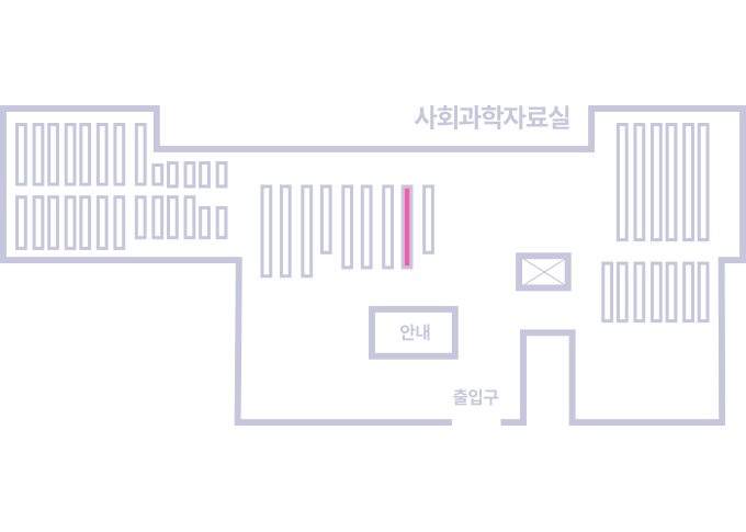
도서위치안내: / 서가번호:
우편복사 목록담기를 완료하였습니다.
*표시는 필수 입력사항입니다.
저장 되었습니다.