대표어
대표어


권호기사보기
| 기사명 | 저자명 | 페이지 | 원문 | 기사목차 |
|---|
결과 내 검색
동의어 포함
목차
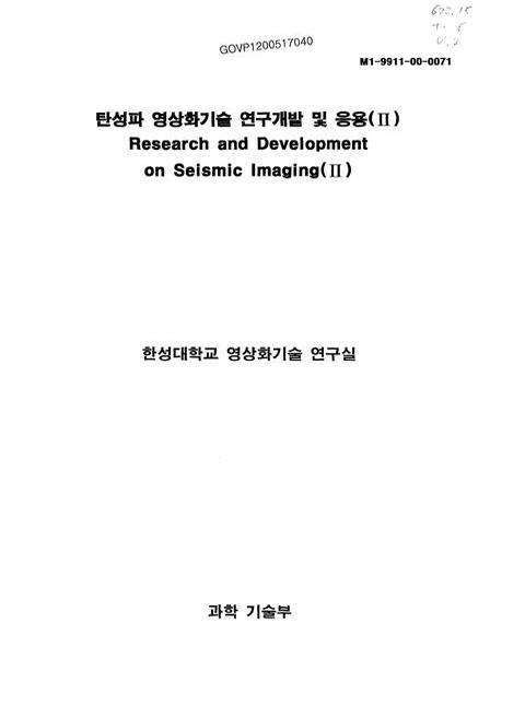
[표제지 등]=0,1,2
제출문=1,3,1
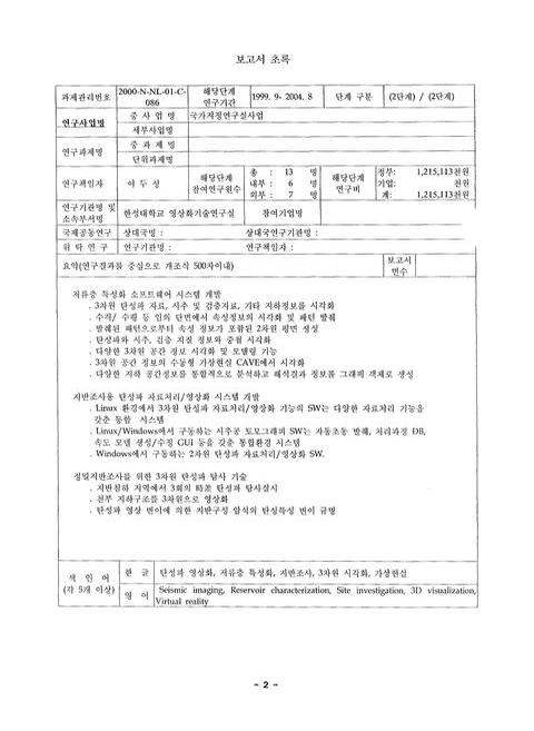
보고서 초록=2,4,1
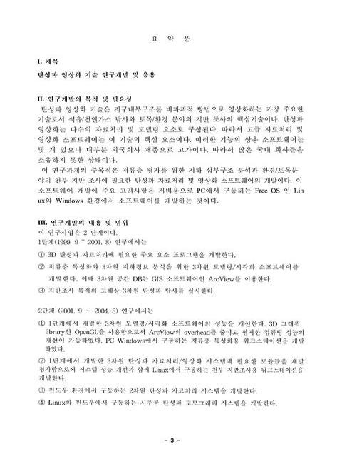
요약문=3,5,8
목차=11,13,2
제1장 연구개발과제의 개요=13,15,3
제2장 국내외 기술개발 현황=16,18,1
제3장 연구개발 수행내용 및 결과=17,19,1
제1절 탄성파 자료처리 시스템 개발=18,20,1
3-1-1. 3차원 탄성파 자료처리 시스템 (ISU3D)=18,20,16
3-1-2. 2차원 자료처리 시스템 (Seispro)[원문불량;p.37]=34,36,7
3-1-3. 시추공 탄성파 토모그래피 소프트웨어(EZTOMO)=41,43,11
제2절 3차원 시각화 시스템 개발(SeisView)=52,54,1
3-2-1. GOCAD를 이용한 저류층 속성정보의 3차원 시각화 기술=52,54,13
3-2-2. ArcView 환경의 3차원 시각화=65,67,3
제3절 SeisView3D system=68,70,3
3-3-1. 층준 시각화=71,73,2
3-3-2. 검층 자료 시각화=73,75,3
3-3-3. 가상현실 환경 시각화 시스템 개발=76,78,5
제4절 시차 3차원 탄성파 탐사=81,83,3
3-4-1. 3차원 시차 탄성파 자료의 처리 및 해석=84,86,4
3-4-2. 시차 3차원 탄성파를 이용한 지반침하 해석=88,90,4
제5절 시추공 토모그래피 탐사=92,94,1
3-5-1. 탐사 방법 및 결과=92,94,9
3-5-2. 3차원 시추공간 토모그래피 및 구조보정=101,103,3
3-5-3. P파, S파 속도 영상도출=104,106,6
제6절 SeisView3D를 이용한 3차원 시각화 사례=110,112,1
3-6-1. Boonsville 3D seismic and well log시각화=110,112,6
3-6-2. 물리탐사 자료 3차원 시각화=116,118,4
제4장 목표달성도 및 관련분야 기여도=120,122,1
제1절 저류층 특성화 워크스테이센 개발=120,122,1
제2절 탄성파 기반 지반조사 워크스테이션 개발=121,123,1
제3절 탄성파 영상화 기술 및 고해상 지반 조사=122,124,1
제5장 연구개발 결과의 활용계획=123,125,1
제6장 연구개발 과정에서 수집한 해외 과학기술정보=124,126,1
제7장 참고문헌=125,127,5
부록 A=130,132,1
1. SeisView3D 사용자 메뉴얼=130,132,1
목차=131,133,2
제1장 Horizon=133,135,1
1. Creating Horizon=133,135,1
1) Creating From Seismic Picking=133,135,2
2. Picking=135,137,5
3. Creating Plane=140,142,1
4. Creating Well Path=141,143,2
5. Data Frame=143,145,1
1) Data Frame=143,145,1
2) Data Frame Option=144,146,3
6. Color Space=147,149,2
7. Color Legend=149,151,1
1) Color Legend=149,151,2
2) Color Legend Option=150,152,2
8. Picked Point Option=152,154,2
9. Contour=154,156,3
제2장 Well Log=157,159,1
1. Creating Well Log In 3D Window=157,159,1
1. 하나의 Well Log Data 입력=157,159,2
2. Selecting Coordinate=159,161,2
3. Displaying Well Log=161,163,1
4. 다중의 Well Log Data 입력=161,163,2
2. Selecting Well Log=163,165,1
1. Selecting=163,165,1
2. Lasso Representation=163,165,1
3. Lasso Policy Field=163,165,2
3. Showing Vertical Coordinate Values=165,167,2
4. Changing Radius=167,169,1
5. Changing Color=167,169,2
6. Displaying Well Log In 2D Window=169,171,1
1. Showing Well Name And Coordinate Values (x, y)=170,172,1
2. Picking Well Log=171,173,1
3. Displaying Well Log in Line=171,173,2
4. Showing Well Name And Depth Value=172,174,1
7. Creating Horizon In 2D Window=173,175,1
1) Picking=173,175,2
2) Editing=175,177,2
3) Saving Horizon=177,179,6
4) Loading Horizon=183,185,1
8. Creating Horizon From Log Picking In 3D Window=184,186,1
1) Thin Plate Spline=184,186,2
2) Kriging=186,188,2
9. Changing Axes Scale=188,190,2
10. Cloaking Well Log=190,192,2
11. Deleting Well Log Selected=192,194,2
제3장 Volume=194,196,1
탄성파 자료 시각화=194,196,1
1. Creating Volume=194,196,1
1) 자료 입력=194,196,4
2) 음영 효과 (Shade effect)=197,199,4
2. Moving Slices=201,203,2
3. Horizon Picking=203,205,2
일반 볼륨 자료 시각화=205,207,1
1. Creating Volume From Text File=205,207,2
2. Rendering Whole Volume=207,209,3
3. Creating Other Volume From Volume Picking=210,212,5
영문목차
[title page etc.]=0,1,7
Summary=6,8,3
Contents=9,11,4
Chapter 1. Introduction=13,15,3
Chapter 2. State Of Research And Development=16,18,1
Chapter 3. Contents And Results Of The Research And Development=17,19,1
Section 1. Development Of Seismic Data Processing / Imaging System=18,20,1
3-1-1. 3D Seismic Data Processing/Imaging System (lSU3D)=18,20,16
3-1-2. 2D Seismic Data Processing System (Seispro)[원문불량;p.37]=34,36,7
3-1-3. Crosswell Seismic Tomography Software (EZTOMO)=41,43,11
Section 2. 3D Visualization System=52,54,1
3-2-1. 3D Visualization Of Reservoir Attributes Using The GOCAD=52,54,13
3-2-2. 3D Modeling/ Visualization Using The SeisView=65,67,3
Section 3. SeisView3D System=68,70,3
3-3-1. Horizon Visualization=71,73,2
3-3-2. Well-log Visualization=73,75,3
3-3-3. Virtual Reality Display System=76,78,5
Section 4. Time Lapse 3D Seismic Survey=81,83,3
3-4-1. Data Processing=84,86,4
3-4-2. Evaluation Of The Ground Subsidence Using The Time Lapse 3D Seismic Method=88,90,4
Section 5. Crosswell Seismic Survey=92,94,1
3-5-1. Travel-time Crosswell Tomography=92,94,9
3-5-2. Migration Study On The Crosswell Seismic Data=101,103,3
3-5-3. P-S Wave Velocity Tomogram=104,106,6
Section 6. Visualization Using The SeisView3D=110,112,1
3-6-1. Visualization Of The Boonsville 3D Seismic And Well Logs=110,112,6
3-6-2. Visualization Of The Electrical Survey Data=116,118,4
Chapter 4. Achievement Snd Contribution=120,122,1
Section 1. Development Of A Workstation For Reservoir Characterization=120,122,1
Section 2. Development Of A Seismic Based Workstation For Site investigation=121,123,1
Section 3. High Resolution Seismic Imaging Technology For The Engineering problem=122,124,1
Chapter 5. Application Plan Of The Results=123,125,1
Chapter 6. Recent Information Of Science And Technology=124,126,1
Chapter 7. References=125,127,5
Appendix A=130,132,1
1. SeisView3D User's Manual=130,132,85
jpg
Fig. 3-2-12. Integrated 3-D Visualization Of Coherence Cube (value<O.3), 38 Well Logs, And 4 Horizons. Coherence Values On Each Surface Are Represented From Red (low) To White (high)=61,63,1
Fig. 3-3-4. The Horizons Created By Picking Seismic Volume Data. Colors Are Assigned By Seismic Amplitudes On A Position Of Each Points=71,73,1
Fig. 3-3-5. A Surface Created By Interpolating Picked Points For Linear Features On Two Horizons. The Red Points Are Assigned As Datum Points To Control The Shape Of The Surface By Connecting Them=72,74,1
Fig. 3-3-6. A Well Path Created On A Surface Between Two Horizons=72,74,1
Fig. 3-3-9. The Horizons Created By TPS Interpolation (colored) Are Superposed On Horizons Created From Seismic Picks (grayscale)=75,77,1
Fig. 3-3-13. A Stereoscopic Image Of The Two Seismic Horizons Projected On A CAVE Environment=80,82,1
Fig. 3-4-3. Geological Drill Log=84,86,1
Fig. 3-5-10. (a) Theoretical Velocity Model and (b) Example Display Of Fresnel Volume(shot (0,0,8), Receiver (10,20,34)) (c) 3D Tomogram=103,105,1
Fig. 3-5-13. S Wave First Arrivals (troughs) Are Picked On A Common Receiver Gather. F-K And High Cut Filters Are Applied=108,110,1
Fig. 3-5-14. P Wave Velocity Tomograms. From Lett Section 1, Section 2, And Section 3. Section 1 Crosses An Empty Tunnel And Sections 2 And 3 Are Crossing The Tunnel Filled By Sands And Rock Debris, Respectively. The Distance Unit Is cm=108,110,1
Fig. 3-5-15. S Wave Velocity Tomograms. From Lett Section 1, Section 2, and section 3=109,111,1
Fig. 3-5-16. Tomograms Showing Velocity Ratios, Vp/Vs. From Left Section 1, Section 2 , And Section 3=109,111,1
Fig. 3-6-1. 3차원 탄성파 자료의 볼륨 시각화=110,112,1
Fig. 3-6-2. Dragger를 이용한 단면 이동=111,113,1
Fig. 3-6-3. Horizon 발췌=111,113,1
Fig. 3-6-4. 반투명 효과=112,114,1
Fig. 3-6-5. 단층선 추출=112,114,1
Fig. 3-6-6. 단층명 생성=112,114,1
Fig. 3-6-10. 탄성파로부터 생성된 Horizon (고주파) 과 검층기록으로부터 생성한 Horizon을 중첩하여 Display한 예=114,116,1
Fig. 3-6-11. 3차원 탄성파볼륨, 검층 등을 중첩하여 Display=115,117,1
Fig. 3-6-12. 물리탐사 측선을 표시한 도면=115,117,1
Fig. 3-6-13. 각 측점에서 획득한 Sp Data를 지표의 토포그래피를 도시한 예=116,118,1
Fig. 3-6-14. 비저항 데이터를 볼륨으로 도시=116,118,1
Fig. 3-6-15. 수직/수평단면 상의 비저항을 도시=117,119,1
Fig. 3-6-16. 저 비저항대를 칼라로 표시=117,119,1
Fig. 3-6-17. 비저항 볼륨과 비저항 토모그래피 이미지를 중첩하여 도시=118,120,1
Fig. 3-6-18. 비저항 볼륨의 Color값을 바꾸어서 도시=118,120,1
Fig. 3-6-19. 비저항 볼륨을 반투명으로 비저항 토모그래피와 중첩하여 도시=118,120,1
Fig. 3-6-20. 저비저항대를 3차원으로 생성=119,121,1
Figure 1-2. 파일 열기 대화 상자에서 파일을 선택한 모습=134,136,1
Figure 1-3. 화면에 그려진 Horizon=134,136,1
Figure 2-1. Picking 실행 초기 화면=135,137,1
Figure 2-2. Picking을 통한 포인트 생성=136,138,1
Figure 2-3. Picking 종료 화면=136,138,1
Figure 2-4. 생성된 포인트 지우기=137,139,1
Figure 2-5. 포인트 추가=137,139,1
Figure 2-6. 포인트의 위치 변경 (전)=138,140,1
Figure 2-7. 포인트의 위치 변경 (후)=138,140,1
Figure 2-8. Datum Point 설정 - 각 Horizon에 2개씩의 Datum Point를 지정하고 있다=139,141,1
Figure 4-3. Plane에 투명도 적용 화면=142,144,1
Figure 5-1. [Data Frame]메뉴를 선택=143,145,1
Figure 5-2. Horizon에 대한 Data Frame 생성=143,145,1
Figure 5-4. Show Axes Title=145,147,1
Figure 5-5. Show Axes Title and Show Tick Label=145,147,1
Figure 5-6. Show Grid Line=146,148,1
Figure 6-1. Color Space=147,149,1
Figure 6-2. 초기 대화 상자=147,149,1
Figure 6-3. 설정 후 대화 상자=147,149,1
Figure 6-4. Color Model의 적용=148,150,1
Figure 7-1. Horizon의 선택=149,151,1
Figure 7-2. Color Legend=149,151,1
Figure 7-3. 선택 시 변화된 Color Legend=150,152,1
Figure 7-4. Color Legend Option=150,152,1
Figure 7-5. 대화 상자의 값 수정=151,153,1
Figure 7-6. 변화된 Color Legend=151,153,1
Figure 8-1. 변화 된 Color Legend=152,154,1
Figure 8-2. 초기 대화 상자=152,154,1
Figure 8-3. 설정 후 대화 상자=152,154,1
Figure 8-4. 수정 된 Point=153,155,1
Figure 9-1. Create Contour=154,156,1
Figure 9-2. 초기 대화 상자=154,156,1
Figure 9-3. 설정 후의 대화 상자=154,156,1
Figure 9-4. Horizon위에 그려진 등고선=155,157,1
Figure 9-5. Horizon위에 그려진 등고선=155,157,1
Figure 1-4. 화면에 그려진 Volume=197,199,1
Figure 1-5. [Volume] 메뉴의 [Shade Slices]=197,199,1
Figure 1-6. 음영효과가 적용된 Volume=198,200,1
Figure 1-7. [Lights]의 서브 메뉴에 [Headlight]-[Edit]...선택=198,200,1
Figure 1-8. Headlight Editor 대화상자=199,201,1
Figure 1-9. [Lights]의 서브 메뉴에 [Create Point Light] 선택하는 모습=199,201,1
Figure 2-3. 드래거로 단면을 움직이는 예=202,204,1
Figure 2-4. 특정한 값만 가진 부위만 도시된 예=209,211,1
Figure 2-5. MRI 자료를 도시한 예=209,211,1
Figure 3-8. Material Editor 대화 상자=214,216,1
Figure 3-9. surface에 색 정보를 준 후 도시된 예=214,216,1
| 등록번호 | 청구기호 | 권별정보 | 자료실 | 이용여부 |
|---|---|---|---|---|
| 0001080916 | 622.15 ㄱ373ㅌ | v.2 | 서울관 서고(열람신청 후 1층 대출대) | 이용중 |
| 0001080917 | 622.15 ㄱ373ㅌ | v.2 | 서울관 서고(열람신청 후 1층 대출대) | 이용중 |
*표시는 필수 입력사항입니다.
| 전화번호 |
|---|
| 기사명 | 저자명 | 페이지 | 원문 | 기사목차 |
|---|
| 번호 | 발행일자 | 권호명 | 제본정보 | 자료실 | 원문 | 신청 페이지 |
|---|
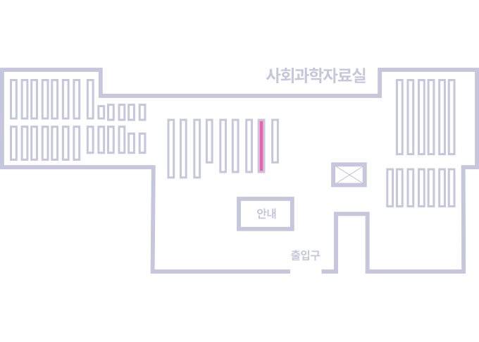
도서위치안내: / 서가번호:
우편복사 목록담기를 완료하였습니다.
*표시는 필수 입력사항입니다.
저장 되었습니다.