대표어


권호기사보기
| 기사명 | 저자명 | 페이지 | 원문 | 기사목차 |
|---|
결과 내 검색
동의어 포함
목차
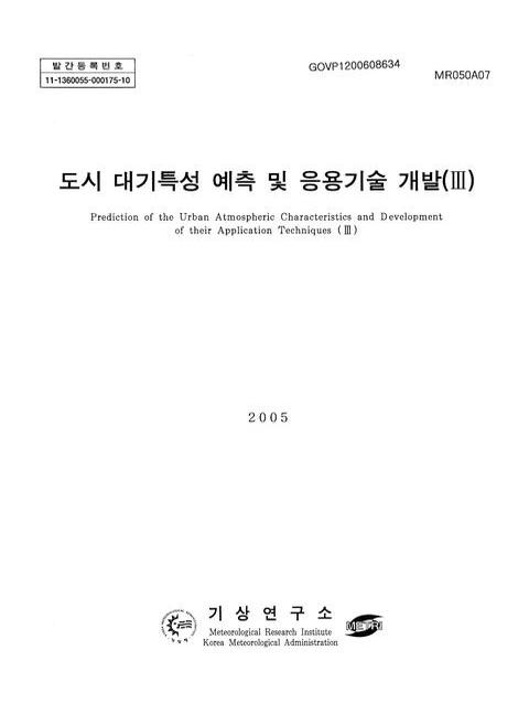
[표제지 등]=0,1,2
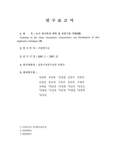
연구보고서=0,3,1
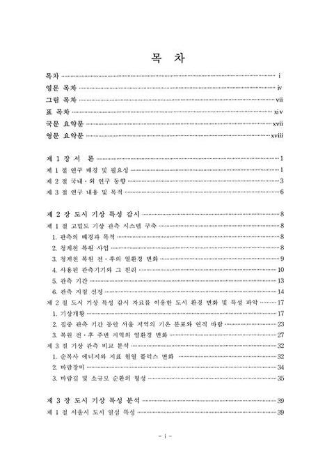
목차=i,4,3
Contents=iv,7,3
List Of Figures=vii,10,7
List Of Tables=xiv,17,3
요약문=xvii,20,1
Summary=xviii,21,2
제1장 서론=1,23,1
제1절 연구 배경 및 필요성=1,23,3
제2절 국내ㆍ외 연구 동향=3,25,3
제3절 연구 내용 및 목적=6,28,2
제2장 도시 기상 특성 감시=8,30,1
제1절 고밀도 기상 관측 체계 구축=8,30,1
1. 관측의 배경과 목적=8,30,1
2. 청계천 복원 사업=8,30,2
3. 청계천 복원 전ㆍ후의 열환경 변화=9,31,1
4. 사용된 관측기기와 그 원리=10,32,4
5. 관측=13,35,2
6. 관측 지점 선정=14,36,3
제2절 도시 기상 특성 감시 자료를 이용한 도시 환경 변화 및 특성 파악=17,39,1
1. 기상개황=17,39,6
2. 집중 관측 기간 동안 서울 지역의 기온 분포와 연직 바람=23,45,5
3. 복원 전ㆍ후 주변 지역의 열환경 변화=27,49,5
제3절 기상 관측 비교 분석=32,54,1
1. 순복사 에너지와 지표 현열 플럭스 변화=32,54,2
2. 바람장미=34,56,1
3. 바람길 및 소규모 순환의 형성=35,57,4
제3장 도시 기상 특성 분석=39,61,1
제1절 서울시 도시 열섬 특성=39,61,1
1. 개요=39,61,2
2. 자료 및 분석 방법=40,62,5
3. 결과=44,66,11
제2절 도심 열환경 평가를 위한 열수지 모델의 적용 및 검증=55,77,1
1. 개요=55,77,1
2. 연구 방법=56,78,3
3. 결과 및 고찰=58,80,9
제3절 바람분포에 의한 서울 강우 특성=67,89,1
1. 개요=67,89,2
2. 자료 및 방법=68,90,2
3. 분석 결과=69,91,12
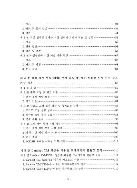
제4장 전산 유체 역학(CFD) 모형 개발 및 이를 이용한 도시 지역 상세 기상 예측=81,103,1
제1절 개요=81,103,1
제2절 수치 모형 및 접합 기술=82,104,1
1. 전산 유체 역학 모형=82,104,3
2. 접합 기술=84,106,3
제3절 중규모 모형 결과 검증 및 국지순환 분석=86,108,1
1. 중규모 모형 실험 설계=86,108,3
2. 중규모 모형 결과 검증=88,110,5
3. 국지 순환 분석=92,114,7
제4절 도시 지역 상세 기상 예측=98,120,1
1. 전산 유체 역학 모형 실험 설계=98,120,3
2. 상세 기상 예측 결과 및 토의=100,122,9
3. 건물 효과=109,131,3
4. SODAR 자료를 이용한 모형 실험=112,134,2
제5장 Landsat TM 영상을 이용한 도시지역의 열환경 분석=114,136,1
제1절 Landsat TM/ETM+ 영상을 이용한 도시지역의 열환경 분석=114,136,1
1. Landsat TM band 6을 이용한 지표온도 추출=114,136,4
2. Landsat TM/ETM+를 이용한 토지피복분포도 작성=117,139,3
3. Landsat TM/ETM+를 이용한 정규식생지수 분석=119,141,2
제2절 ASTER 영상을 이용한 도시지역의 열환경 분석=121,143,1
1. 연구자료 및 방법=121,143,11
제3절 위성영상 자료를 이용한 도시지역의 열환경 분석=132,154,1
1. 위성영상자료의 전 처리=132,154,3
2. ASTER TIR센서를 이용한 지표 열환경 분석=135,157,5
3. ASTER VNIR센서를 이용한 정규식생지수(Normalized Difference Vegetation Index) 분석=140,162,4
4. 토지피복 분류를 통한 지표온도 특성 분석=144,166,13
제4절 GIS 공간 분석을 이용한 도시환경 특성 분석=157,179,1
1. GIS(Geographic Information System)의 개요=157,179,5
2. 지표온도 분포도와 AWS자료의 중첩분석을 통한 상관성 분석=162,184,2
3. 근접성 분석에 따른 청계천 주위 온도 및 식생활력 분포 특성=163,185,2
4. 정규식생지수와 지표온도와의 상관성 분석=165,187,2
제6장 요약 및 결론=167,189,1
제1절 연구 결과 종합=167,189,4
제2절 기대효과 및 활용방안=171,193,1
제7장 참고 문헌=172,194,7
Fig. 2.1. The Pictures Taken By Thermography Of Thermal Environment Change For The (a) Before (2003) And (b) After (2004) Restoration Of Cheonggye Stream=9,31,1
Fig. 2.2. Meteorological Observation Instruments Used In This Study=13,35,1
Fig. 2.3. Meteorological Observatories In The Cheonggye Stream Area=15,37,1
Fig. 2.4. Diurnal Variations Of Meteorological Elements (a) From 19 To 26 June 2003 (b) From 10 To 17 August 2003=18,40,2
Fig. 2.5. Diurnal Variations Of Meteorological Elements From 8 To 15 August 2004=20,42,1
Fig. 2.6. Diurnal Variations Of Meteorological Elements (a) From 8 To 11 August 2005 (b) From 22 To 29 September 2005=21,43,2
Fig. 2.7. Distribution Of (a) Averaged Air Temperature And (b) The Differences Between Hourly Data And Hourly Average Data For August 9-13, 2003 In Seoul. The Contour Interval Is 0.5℃=23,45,1
Fig. 2.8. Distribution Of (a) Averaged Air Temperature And (b) The Differences Between Hourly Data And Hourly Average Data For August 9-13, 2004 In Seoul. The Contour Interval Is 0.5℃=24,46,1
Fig. 2.9. Distribution Of (a) Averaged Air Temperature And (b) The Differences Between Hourly Data And Hourly Average Data For August 14-16, 2005 In Seoul. The Contour Interval Is 0.5℃=24,46,1
Fig. 2.10. Distribution Of Temperature In The Cheonggye Stream Area ((a) 12-14 August 2003 (b) 10-13 August 2004 (c) 14-16 August 2005)=25,47,1
Fig. 2.11. Vertical Profiles Of U, V Components And Potential Temperature On 13 August 2003=26,48,1
Fig. 2.12. Vertical Profiles Of U, V, W Components And Wind Speed On 23 September 2005=27,49,1
Fig. 2.13. Distribution Of The Air Temperature Deviation In The Cheonggye Stream Area ((a)2003. 8. 12-14, (b) 2004. 8. 10-13, (c) 2005. 8. 14-16, (d) 2005. 9. 27-28). The Contour Interval Is 0.2℃=28,50,1
Fig. 2.14. Distribution Of The Air Temperature Deviation Between Air Temperature Of 14 Points Of Cheonggye Stream Area And Averaged Air Temperature Of 32 Automatic Weather Station=29,51,1
Fig. 2.15. Diurnal Variations Of The Air Temperature Deviation Between Averaged Air Temperature Of 14 Points Of Cheonggye Stream Area And Averaged Air Temperature Of 32 Automatic Weather Station=30,52,1
Fig. 2.16. Distribution Of The Air Temperature Deviation Between Air Temperature Of 13 Points Of Cheonggye Stream Area And Averaged Air Temperature Of 32 Automatic Weather Station=31,53,1
Fig. 2.17. Diurnal Variations Of The Air Temperature Deviation Between Averaged Air Temperature Of 14 Points Of Cheonggye Stream Area And Averaged Air Temperature Of 32 Automatic Weather Station=31,53,1
Fig. 2.18. Distribution Of The Net Radiation And Sensible Heat In The Cheonggye Stream Area In (a) 2003 And (b) 2005=33,55,1
Fig. 2.19. Windrose Plot In The Cheonggye Stream Area And Seoul Meteorological Observation Station=34,56,1
Fig. 2.20. (a) U, (b) V, (c) W Components Of The Wind And (d) Wind Speed In The Cheonggye Stream Area=36,58,2
Fig. 2.21. Schematic Diagram Of The Wind Circulation In The Cheonggye Stream Area=38,60,1
Fig. 3.1. Locations Of The Automatic Weather Stations (AWSs) In The Seoul Metropolitan Area. The Boundary Between Seoul And Its Surrounding Regions Is Indicated By A Thick Solid Line And Topography Is Shaded With Different Scales=41,63,1
Fig. 3.2. Land-Use Map In The Seoul Metropolitan Area Constructed Using Geographic Information System (GIS). Seoul Is Divided Into 25 Administrative Subregions, Called Gu In Korean, Which Are Demarcated By Solid Lines. This Map Is For April 1999=44,66,1
Fig. 3.3. Distribution Of Air Temperature Averaged For The One-Year Period Of March 2001 To February 2002. The Contour Interval Is 0.2℃=45,67,1
Fig. 3.4. Distribution Of Air Temperature Averaged For Each Hour Of March 2001 To February 2002. The Plots Are Given In 3-Hour Intervals. The Contour Interval Is 0.2℃=47,69,1
Fig. 3.5. Time Series Of Difference Between Air Temperature At Seocho And Three-Station Averaged Temperature At (a) 03, (b) 09, (c) 15, And (d) 21 LST. The Three Stations Are Sanung, Nunggok, And Goyang=48,70,1
Fig. 3.6. Temporal Behavior Of The First And Second Empirical Orthogonal Functions (EOFS) For Air Temperatures Averaged For Each Hour Of March 2001 To February 2002=49,71,1
Fig. 3.7. Spatial Display Of The First And Second Empirical Orthogonal Functions (EOFS) For Air Temperatures Averaged For Each Hour Of March 2001 To February 2002. The Contour Interval Is 0.1℃=50,72,1
Fig. 3.8. Distribution Of Precipitation, Wind Speed, Minimum Air Temperature, And Maximum Air Temperature Averaged For The Summertime Of June 2003 To August 2003=51,73,1
Fig. 3.9. Distribution Of (a) Air Temperature And (b) Air Temperature Including 12 Points In The Cheonggye Stream Area Averaged For The Summertime Of June 2003 To August 2003. + Denote The Measurement Points Of Air Temperature And Relative Humidity In The Cheonggye Stream Area. The Contour Interval Is 0.5℃=53,75,1
Fig. 3.10. Time Series Of Difference Between Air Temperature At 12 Stationary Points In The Cheonggye Stream Area And Eight-Station In Suburb Area Averaged Temperature At (a) 03, (b) 09, (c) 15, And (d) 21 LST=54,76,1
Fig. 3.11. Schematic Diagram Of Heat Budget Model For Surface (After 近藤 (1992))=56,78,1
Fig. 3.12. Observation Sites For Measurement Of Surface Energy Flux And Meteorological Data. For Land Cover Type, Haenam Site Is A Grassy Area And Seoul Site To Be At The Building Top (Elementary School) Of City Center Is A Concrete=57,79,1
Fig. 3.13. Surface Energy Flux, To Be Observed The Period Of (a) Jul.-Aug., (b) Sep.-Oct. And (c) Nov.-Dec. 2002, For Grassy Place At Haenam. Sg, Represents Shortwave Radiative Flux, Rg, Longwave Radiative Flux, S.H. Sensible Heat Flux, L.H. Latent Heat Flux=59,81,1
Fig. 3.14. Comparison Between Downward And Upward Shortwave Radiative Fluxes For Grassy Place At Haenam. The Periods Are (a) Jul.-Aug., (b) Sep.-Oct. And (c) Nov.-Dec. 2002. The Slope Of The Line Represents The Albedo=60,82,1
Fig. 3.15. Comparison Of Observed And Calculated Energy Flux, (a) Upward Shortwave Radiative Flux, (b) Upward Longwave Radiative Flux, (c) Sensible Heat Flux And (d) Latent Heat Flux, For Grassy Field At Haenam. The Period Is Jul.-Aug. 2002=61,83,1
Fig. 3.16. The Same As Fig. 3.15 Except For Sep.-Oct. 2002=62,84,1
Fig. 3.17. The Same As Fig. 3.15 Except For Nov.- Dec. 2002=62,84,1
Fig. 3.18. Surface Energy Flux, To Be Observed The Period Of 12-13 August 2003 For Built-Up Area At Seoul. Sg Represents Shortwave Radiative Flux, Rg Longwave Radiative Flux, S.H. Sensible Heat Flux=64,86,1
Fig. 3.19. Comparison Between Downward And Upward Shortwave Radiative Fluxes For Built-Up Area In Seoul. The Data'S Period Is A Jul.-Aug. 2003. The Slope Of The Line Represents The Albedo=64,86,1
Fig. 3.20. Comparison Of Observed And Calculated Energy Flux, (a) Upward Shortwave Radiative Flux, (b) Upward Longwave Radiative Flux And (c) Sensible Heat Flux, For Built-Up Area In Seoul. The Period Is 12-13 Aug. 2003=65,87,1
Fig. 3.21. Comparison Of The Built-Up Area And Assumed Grassy Place For Calculated Surface Temperature=66,88,1
Fig. 3.22. Horizontal Distribution Of Annual Precipitation In Seoul, 1998-2004=70,92,1
Fig. 3.23. Variation In Number Of Days With Heavy Rainfall (≥20 mmhr-¹) Every Year At Each Station=71,93,1
Fig. 3.24. Total Seasonal Precipitation (mm) For Each Pre-Event Flow Direction (Shown As Arrows), 1998-2004. The Red Letter Represents Precipitation Of The Downwind Area=73,95,1
Fig. 3.25. Total Seasonal Precipitation Events (Days) For Each Pre-Event Flow Direction (Shown As Arrows), 1998-2004. The Red Letter Represents Precipitation Of The Downwind Area=75,97,1
Fig. 3.26. Quadrant Precipitation (mm) And Precipitation Events (Days) For Each Season Based On The Combining Quadrant Values In All Events Based On Pre-Event Wind Flow Direction (Shown As Arrows). The Red Letter Represents Precipitation Of The Downwind Area=77,99,1
Fig. 3.27. Quadrant Precipitation (mm) And Precipitation Events (Days) During Summer Season Based On Combining Quadrant Values In Events Over 20 mmhr-¹ Based On Pre-Event Wind Flow Direction (Shown As Arrows). The Red Letters Represent Values Of The Downwind Areas=78,100,1
Fig. 3.28. Quadrant Precipitation (mm) And Precipitation Events (Days) During Summer Season Based On Combining Quadrant Values In All Events Over 20 mmhr-¹ Based On The Pre-Event Wind Flow Direction (Shown As Arrows). The Red Letters Represent Values Of The Downwind Areas=78,100,1
Fig. 4.1. Schematic Of Vertical Levels Of Interpolation Method=85,107,1
Fig. 4.2. Model Domain In MM5 Simulation=87,109,1
Fig. 4.3. Simulated And Observed Sea-Level Pressure Fields At 00UTC 1 June 2004=89,111,1
Fig. 4.4. Simulated And Observed Sea-Level Pressure Fields At 00UTC 2 June 2004=90,112,1
Fig. 4.5. Time Series Of (a) Temperature At Height Of 2 m In The Case Of Simulation And 1.5 m In The Case Of Observation, And (b) Time Series Of Wind Speed At A Height Of 10 m=90,112,1
Fig. 4.6. Time Series Of (a) Simulated Temperature And AWS Observed Temperature And (b) Simulated Wind Speed And AWS Observed Wind Speed At Secho AWS Station, And Time Series Of (c) Simulated Temperature And AWS Temperature And (d) Simulated Wind Speed And AWS Wind Speed At Kangdong AWS Station=91,113,1
Fig. 4.7. Time Series Of (a) Simulated Temperature And AWS Observed Temperature And (b) Simulated Wind Speed And AWS Observed Wind Speed At Kangseo AWS Station, And Time Series Of (c) Simulated Temperature And AWS Temperature And (d) Simulated Wind Speed And AWS Wind Speed At Dongdaemun AWS Station=92,114,1
Fig. 4.8. Wind Field In Domain 4 At 18UTC 2 June 2004=94,116,1
Fig. 4.9. Wind Field In Domain 4 At 00UTC 2 June 2004=94,116,1
Fig. 4.10. Wind Field In Domain 4 At 06Utc 2 June 2004=95,117,1
Fig. 4.11. Wind Field In Domain 4 At 12Utc 2 June 2004=95,117,1
Fig. 4.12. Wind Field In Domain 4 At 18Utc 2 June 2004=96,118,1
Fig. 4.13. 10 m Wind Field Around The CFD Domain At (a) 12UTC 1 June 2004, And At (b) 18UTC 1 June 2004=97,119,1
Fig. 4.14. 10 m Wind Field Around The CFD Domain At (a) 00UTC 2 June 2004, And At (b) 06UTC 2 June 2004, (c) 12Utc 2 June 2004, And (d) 18UTC 2 June 2004=97,119,1
Fig. 4.15. Map Of Cheonggye Stream Area Constructed Using Geographic Information System (GIS)=99,121,1
Fig. 4.16. Model Domain And Building Configuration In This Study=100,122,1
Fig. 4.17. Wind Vector Fields At (a) Z=2.5 m And (b) Z=17.5 m At 01UTC 2 June 2004=102,124,1
Fig. 4.18. Wind Vector Fields At (a) Z=2.5 m And (b) Z=17.5 M At 03UTC 2 June 2004=103,125,1
Fig. 4.19. Wind Vector Fields At (a) Z=2.5 m And (b) Z=17.5 M At 04UTC 2 June 2004=105,127,1
Fig. 4.20. Wind Vector Fields At (a) Z=2.5 m And (b) Z=17.5 M At 06UTC 2 June 2004=106,128,1
Fig. 4.21. (a) Wind Vector Fields At Z=17.5 m At 06UTC 2 June 2004 And Three Characteristic Flow Regimes, (b) Channeling Flow, (c) Double-Eddy Circulation, And (d) Recirculation Zone=108,130,1
Fig. 4.22. Vertical Profile Of Wind Speed Of MM5 And CFD At 01UTC 2 June 2004=110,132,1
Fig. 4.23. Vertical Profile Of Wind Speed Of MM5 And CFD At 03UTC 2 June 2004=111,133,1
Fig. 4.24. Vertical Profile Of Wind Speed Of MM5 And CFD At 05UTC 2 June 2004=111,133,1
Fig. 4.25. Wind Vector Fields At (a) Z=2.5 m And (b) Z=17.5 m=113,135,1
Fig. 5.1. Surface Temperature Distribution Map Using Landsat TM/ETM+ Images In Seoul=115,137,1
Fig. 5.2. Curve Pattern Of Temporal Surface Temperature Distribution=115,137,1
Fig. 5.3. Surface Temperature Extraction Considering The Difference Of Temporal Temperature=116,138,1
Fig. 5.4. Land Cover Classification Using Temporal Landsat TM And ETM+=118,140,1
Fig. 5.5. Land Cover Change Graph In Seoul=119,141,1
Fig. 5.6. Temporal NDVI Distribution Map In Seoul=119,141,1
Fig. 5.7. Location Of The Study Area (25 Districts In Seoul)=121,143,1
Fig. 5.8. Study Flow Chart=124,146,1
Fig. 5.9. ASTER VNIR, SWIR, TIR Sensor Images In Seoul=125,147,1
Fig. 5.10. Band Wave Length Of ASTER Images And Standard Product Diagram=127,149,1
Fig. 5.11. AWS Location In Seoul=131,153,1
Fig. 5.12. Electronic Wave Length Of Remote Sensing=135,157,1
Fig. 5.13. Black Body Radiation=136,158,1
Fig. 5.14. Spectral Emissivity And Radiant Flux=137,159,1
Fig. 5.15. Surface Temperature Distribution Using ASTER TIR Data=139,161,1
Fig. 5.16. Surface Temperature Of 25 Districts In Seoul=139,161,1
Fig. 5.17. NDVI Map In Seoul Using Aster Images=143,165,1
Fig. 5.18. Average NDVI Graph Of 25 Districts In Seoul=143,165,1
Fig. 5.19. Land-Cover Classification Map Using ASTER Images In Seoul (2004. 4. 17)=148,170,1
Fig. 5.20. Land-Cover Area Graph Of 25 Districts In Seoul=150,172,1
Fig. 5.21. Surface Temperature Graph Of Each Land-Cover Pattern=150,172,1
Fig. 5.22. High Surface Temperature Distribution Map Using IKONOS=156,178,1
Fig. 5.23. Overlay Analysis=158,180,1
Fig. 5.24. Buffering Of Point, Line And Area=161,183,1
Fig. 5.25. Correlation Of Surface Temperature Between AWS Data And Satellite Images=163,185,1
Fig. 5.26. Connectivity Analysis Of Cheonggye Stream=164,186,1
Fig. 5.27. Average Surface Temperature Of The Cheonggye Stream Area=164,186,1
Fig. 5.28. Sample Data Distribution Map Between NDVI And Surface Temperature=165,187,1
Fig. 5.29. Correlation Analysis Between NDVI And Surface Temperature=166,188,1
*표시는 필수 입력사항입니다.
| 전화번호 |
|---|
| 기사명 | 저자명 | 페이지 | 원문 | 기사목차 |
|---|
| 번호 | 발행일자 | 권호명 | 제본정보 | 자료실 | 원문 | 신청 페이지 |
|---|
도서위치안내: / 서가번호:
우편복사 목록담기를 완료하였습니다.
*표시는 필수 입력사항입니다.
저장 되었습니다.