대표어
대표어
권호기사보기
| 기사명 | 저자명 | 페이지 | 원문 | 기사목차 |
|---|
결과 내 검색
동의어 포함
목차
[표제지]=0,1,1
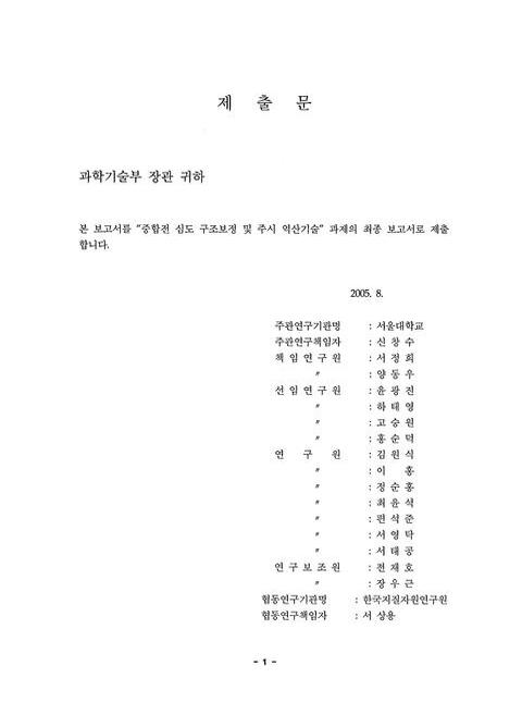
제출문=1,2,2
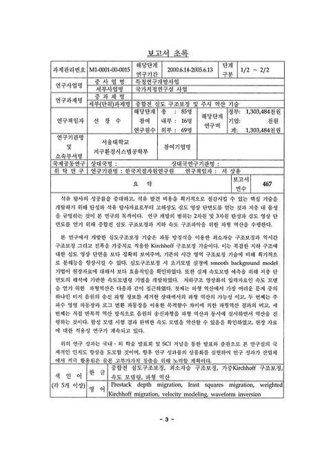
보고서 초록=3,4,1
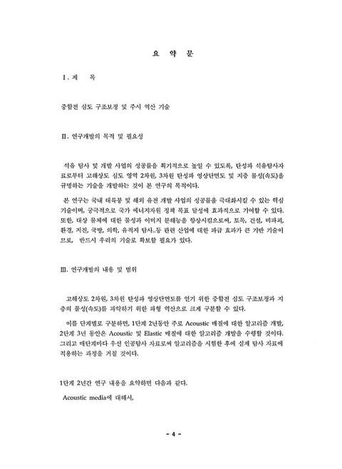
요약문=4,5,5
Summary=9,10,4
Contents=13,14,1
목차=14,15,3
제1장 연구개발과제의 개요=17,18,1
제2장 국내외 기술개발 현황=18,19,3
제3장 연구개발수행 내용 및 결과=21,22,1
제1절 중합전 Kirchhoff 심도 구조보정 기술=21,22,1
3.1.1. 일방향 파동방정식에 의한 초동 주시 및 진폭 계산=21,22,12
3.1.2. 최대에너지 도달 주시 및 진폭 계산=33,34,9
3.1.3. SWEET 알고리즘에 의한 주시 및 진폭 계산=42,43,9
3.1.4. 3차원 SWEET 알고리즘에 의한 주시와 진폭계산=51,52,22
3.1.5. 탄성 매질에서의 주시 및 진폭 계산=73,74,11
3.1.6. 효율적인 주시 및 진폭 계산에 의한 Kirchhoff 심도구조보정=84,85,17
3.1.7. 중합전 Weighted Kirchhoff 심도 구조보정=101,102,12
3.1.8. Smooth Background 중합 전 심도 구조보정=113,114,8
제2절 파동방정식에 기반한 중합전 심도 구조보정 기술=121,122,1
3.2.1. 중합전 최소자승 심도 구조보정=121,122,8
3.2.2. 중합전 2차원 역시간 심도 구조보정=129,130,10
3.2.3. 탄성 매질에서의 중합전 역시간 심도 구조보정=139,140,8
3.2.4. 중합전 3차원 역시간 심도구조보정=147,148,16
제3절 탄성파 파형역산에 의한 속도 모델링 기술=163,164,2
3.3.1. 탄성파 파형역산 이론=165,166,6
3.3.2. 셀분할에 의한 반복적 파형역산=171,172,13
3.3.3. 완전 헤시안 역할 규명에 의한 주파수 영역 파형역산=184,185,6
3.3.4. Pseudo-Multiscale 방식에 의한 파형역산=190,191,18
3.3.5. 주파수 영역 파형역산 알고리즘 비교 Part I=208,209,14
3.3.6. 주파수 영역 파형역산 알고리즘 비교 Part II : Amplitude Approach=222,223,11
3.3.7. 주파수 영역 파형역산 알고리즘 비교 Part III : Phase Approach=233,234,12
3.3.8. 컨벌루션 방식에 의한 송신파형에 독립적인 파형역산=245,246,10
3.3.9. 디컨벌루션 방식에 의한 송신파형에 독립적인 파형역산=255,256,8
3.3.10. 진폭정보만을 이용한 송신파형에 독립적인 파형역산=263,264,13
3.3.11. 로그변환 파동장을 이용한 송신파형에 독립적인 파형역산=276,277,9
3.3.12. 역시간 구조보정 기법을 이용한 전기비저항 역산=285,286,16
제4절 속도 모델링 기술=301,302,1
3.4.1. Interpreter Driven 속도 분석 및 모델링=301,302,20
3.4.2. RMO 속도 분석 및 속도 모델링=321,322,15
제5절 토모그래피 기술=336,337,1
3.5.1. Blocky 반사 주시 토모그래피=336,337,13
3.5.2. 셀 매개변수에 의한 탄성파 반사 주시 토모그래피=349,350,12
3.5.3. SWEET 알고리즘을 이용한 굴절법 토모그래피=361,362,13
3.5.4. 단일 주파수의 감쇄 파동장을 이용한 굴절법 토모그래피=374,375,19
제6절/제5절 위탁과제 : 파형역산 프로그램의 C 언어 변환=393,394,29
제4장 목표달성도 및 관련분야에의 기여도=422,423,4
제5장 연구개발결과의 활용계획=426,427,1
제6장 연구개발과정에서 수집한 해외과학기술정보=427,428,2
제7장 참고문헌=429,430,31
기술요약서(I, II)=460,461,8
영문목차
[title page etc.]=0,1,9
Summary=9,10,4
Contents=13,14,4
Chapter 1. Overview=17,18,1
Chapter 2. Research Trend=18,19,3
Chapter 3. Research Results=21,22,1
Section 3.1. Taveltime Calculation For Kirchhoff Prestack Depth Migration=21,22,100
Section 3.2. Wave Equation Based Prestack Depth Migration=121,122,42
Section 3.3. Velocity Modeling Using Waveform Inversion Techniques=163,164,138
Section 3.4. Velocity Modeling Technique=301,302,35
Section 3.5. Seismic Tomography=336,337,57
Section 3.6. Sub-Project : The C-Language Transformation Of Waveform Inversion Program(INV2D)=393,394,29
Chapter 4. Achievements Of The Objectives And Contributions=422,423,4
Chapter 5. Applicabilities And Future Plan=426,427,1
Chapter 6. Annexed Oversea Technical Information=427,428,2
[Chapter 7. References etc.]=429,430,39
jpg
Fig.3.1.1.2b Absolute Errors Between The Analytic Traveltimes And Those Calculated By Our Algorithm=27,28,1
Fig.3.1.1.3a Marmousi Model With Targeted Anticline Below Faults And Salt Layer=28,29,1
Fig.3.1.1.3b The Most Energetic Traveltime Contours (Black Solid Line) Obtained By Picking Seismograms Generated By The Finite-Difference Solution Of The One Way Wave Equation=28,29,1
Fig.3.1.1.3c The Most Energetic Amplitude Obtained From Finite-Difference Solutions Of The Oneway Wave Equation=29,30,1
Fig.3.1.1.3d Amplitude Computed By Our Algorithm For The Smoothed Marmousi Model=29,30,1
Fig.3.1.1.4a Traveltime Contours. (a) Most Energetic Traveltime(Black Solid Line), (b) Traveltime Computed By First Method(Black Dashed Line) And (c) Traveltime Computed By Second Method(White Solid Line)=30,31,1
Fig.3.1.1.4b Amplitude Computed By Second Method=31,32,1
Fig.3.1.1.5a Traveltime Contours. (a) Most Energetic Traveltime(Black Solid Line), (b) Traveltime Computed By First Method(Black Dashed Line) And (c) Traveltime Computed By Second Method(White Solid Line)=31,32,1
Fig.3.1.1.5b amplitude Corresponding To The Traveltime Contour Of Fig 3.1.1.4.b=32,33,1
Fig.3.1.2.3. Most Energetic Traveltimes Computed By Our Algorithm(Black Dotted Line) And Pseudo Spectral Method(White Solid Line)=38,39,1
Fig.3.1.2.5. Most Energetic Traveltimes Computed By Our Algorithm(Dotted Line) And Pseudo Spectral Method(Solid Line) For SEG/EAGE Salt Model=39,40,1
Fig.3.1.2.6. Most Energetic Amplitude Corresponding To The Traveltime Contour Of Fig 3.1.2.5=39,40,1
Fig.3.1.2.7. Most Energetic Traveltimes Computed By Our Algorithm(Dotted Line) And Pseudo Spectral Method(Solid Line) For Depth Slice Of SEG/EAGE Salt Model=40,41,1
Fig.3.1.2.8. Most Energetic Amplitude Corresponding To The Traveltime Contour Of Fig 3.1.2.7=40,41,1
Fig.3.1.3.3. (a) Traveltime Contours And (b) Amplitude Image Computed By The SWEET Method For A Two-Layer Model With A Locally Low Velocity Zone=46,47,2
Fig.3.1.3.4. Traveltime Contours Calculated By (a) The SWEET Algorithm And (b) FEM Modeling For The Marmousi Model=48,49,1
Fig.3.1.3.5. Traveltime Contours Computed By the SWEET Algorithm For The Marmousi Model At (a) 0.8 s And (b) 1.1s Overlaid On Snapshot Image Obtained By A FEM Modeling Technique=49,50,1
Fig.3.1.3.6. Amplitude Images Calculated By (a) The SWEET Algorithm And (b) The FEM Modeling Technique For The Mamousi Model=50,51,1
Fig.3.1.4.3. 3-D SEG/EAGE Salt Model=54,55,1
Fig.3.1.4.4. 3 Parallel +Crss-Sections Of 3-D SEG/EAGE Salt Model Of Fig. 3.1.4.3=54,55,1
Fig.3.1.4.5. The Vertical Sliced Velocity Model At The Center Of The 3-D SEG/EAEG Salt Model (x=0, y=6560 m)=55,56,1
Fig.3.1.4.6. The Traveltime Contours Of The First Arrival Wave Events By SWEET Method On A Vertical Slice Of The 3-D SEG/EAEG Salt Velocity Model (x=0, y=6560 m)=56,57,1
Fig.3.1.4.7. The Amplitude Maps Are Superimposed On A Vertical Sliced Traveltime Contours Of 3-D SEG/EAEG Salt Model (x=0, y=6560 m)=56,57,1
Fig.3.1.4.8. Amplitude Image Obtained By FEM Modeling Overlaid With Traveltime Contour By SWEET Algorithm=57,58,1
Fig.3.1.4.9. The Vertical Sliced Velocity Model At The Center Of 3D SEG/EAGE Salt Model (x=3500 m, y=6560 m)=58,59,1
Fig.3.1.4.10. A Point Source Is Located At Left Corner Of Figure 3.1.4.9 The Traveltime Contours Of The First Arrival Wave Events Obtained By SWEET Algorithm On A Vertical Slice Of The 3-D Salt Velocity Model=59,60,1
Fig.3.1.4.11. The Amplitufe Maps The First Arrival Wave Events Obtained By SWEET Algorithm On A Vertical Slice Of The 3-D Salt Velocity Model (Fig. 3.1.4.9)=60,61,1
Fig.3.1.4.12. The Amplitude Maps (Fig. 3.1.4.11) Are Superimposed On A Vertical Sliced Traveltime Contours (Fig. 3.1.4.10) Of 3-D SEG/EAEG Salt Model (x=3500 m, y=6560 m)=61,62,1
Fig.3.1.4.13. The Depth Sliced Velocity Model At The Center Of 3D SEG/EAGE Salt Model (z=1000 m)=62,63,1
Fig.3.1.4.15. The Amplitude Maps The First Arrival Wave Events Obtained By SWEET Algorithm On A Depth Slice Of The 3-D Salt Velocity Model (Fig. 3.1.4.13)=64,65,1
Fig.3.1.4.16. The Traveltime Contours Are Superimposed On The Depth Sliced Amplitude Maps Of 3-D SEG/EAEG Salt Model (z=1000 m). A Point Source Is Located The Center Of x-Axis At Surface=65,66,1
Fig.3.1.4.17. The Vertical Sliced Velocity Model At The Center Of 3D SEG/EAGE Salt Model (x=6560 m)=67,68,1
Fig.3.1.4.18. A Point Source Is Located At The Center Of Figure 3.1.4.17. The Traveltime Contours Of The First Arrival Wave Events Obtained By SWEET Algorithm On A Vertical Slice Of The 3-D Salt Velocity Model=67,68,1
Fig.3.1.4.19. The Amplitufe Maps The First Arrival Wave Events Obtained By SWEET Algorithm On A Vertical Slice Of The 3-D Salt Velocity Model (Fig. 3.1.4.17)=68,69,1
Fig.3.1.4.20. The Amplitude Maps (Fig. 3.1.4.19) Are Superimposed On A Vertical Sliced Traveltime Contours (Fig. 3.1.4.17)=68,69,1
Fig.3.1.5.2. (a) Traveltime Contours, (b) Amplitude Images Of Horizontal Displacement And (c) Amplitude Images Sections Of Vertical Displacement Corresponding To A Horizontal Line Source Of Vertical Force(이미지참조)=77,78,1
Fig.3.1.5.3. Picked Amplitudes Of Horizontal (a) And Vertical (b) Displacement From A Synthetic Seismogram By Time-Domain(이미지참조)=78,79,1
Fig.3.1.5.4. (a) Traveltime contours, (b) Amplitude Of Horizontal Displacement And (c) Amplitude Of Vertical Displacement Corresponding To A Horizontal Line Source Of Horizontal force(이미지참조)=78,79,2
Fig.3.1.5.5. The P-Wave Velocity Distribution Of The Marmousi-2 Model Overlaid With The Traveltime Contours Obtained By Vidale's (1988) Method. (a) Source Located At (x=10.12km, z=0km)(이미지참조)=81,82,1
Fig.3.1.5.6. Amplitude Of Horizontal (c) And Vertical (d) Displacement When A Vertical Source Is Applied For The Marmousi-2 Model Obtained Using The SWEET Algorithm=82,83,1
Fig.3.1.5.7. Traveltime Contours For An Anisotropic Medium. A Horizontal Line Source Of Vertical Force (∫z) Is Located At The Center Of The Model(이미지참조)=83,84,1
Fig.3.1.5.8. Amplitude Maps Of Horizontal (a) And Vertical (b) Displacements For An Anisotropic Medium. A Horizontal Line Source Of Vertical Force(∫z) Is Located At The Center Of The Model(이미지참조)=83,84,1
Fig.3.1.6.3. The Absolute Error Of Traveltime With Respect To Frequency And Damping Factor For Homogeneous Models : (a) v=2km/s And (b) v=8km/s. The Grid Interval Is 8m. The Number Of Grids Is 1151×376=90,91,1
Fig.3.1.6.4. (a) Analytic(Solid Line) And Numerical Traveltimes Computed By Using The Optimum Frequency And Damping Factor(Dotted Line) For The Homogeneous Model Whose Velocity Is 2km/s=91,92,1
Fig.3.1.6.5. Marmousi Model Overlaid By Traveltime Contour Calculated By Using (a) The Method Of Shin et al. (2003a) And (b) The Adaptive Frequency And The Adaptive Damping Factor=94,95,1
Fig.3.1.6.6. (a) Traveltime Contours Calculated By Our Method(Dotted Line) And The Most Energetic Traveltime Contour(Solid Line) Obtained With The Method Used By Shin et al., (2003b) For The Marmousi Model=95,96,1
Fig.3.1.6.7. (a) Traveltime Computed By Our Method For A Three-layer Model, (b) The Transmitted-wave Traveltime Computed Using A One-way Wave Equation=97,98,2
Fig.3.1.6.8. Prestack Kirchhoff Migration Images For The Marmousi Model Using (a) Traveltime Obtained By Our Algorithm And (b) The Most-Energetic Traveltime Obtained By Shin et al., (2003b)=98,99,2
Fig.3.1.6.9. Prestack Kirchhoff Migration Images Generated By Using (a) The Traveltime Obtained By Our Algorithm And (b) The Most Energetic Traveltime Obtained By Shin et al. (2003b) For The Marmousi Model=99,100,2
Fig.3.1.7.1. Marmousi Model With Faults, Salt Layer And Steep Dipping Layers With Velocity Varying From 1500m/s To 5500m/s=105,106,1
Fig.3.1.7.3. Configuration Source And Streamer For Generating The Synthetic Seismogram For Marmousi Model=105,106,1
Fig.3.1.7.4. Unmigrated Stack Section For Marmousi Model=106,107,1
Fig.3.1.7.5. Kirchhoff Prestack Depth Migreated Images For Marmousi Model By Using (a) Vidale's Traveltime, (b) Oneway Traveltime=107,108,1
Fig.3.1.7.6. Kirchhoff Prestack Depth Migreated Image For Marmousi Model By Using Oneway Travel Time And Amplitude Obtained By First Derivative=108,109,1
Fig.3.1.7.7. Kirchhoff Prestack Depth Migreated Images For Marmousi Model By Using (a) Maximum Energy Traveltime, (b) Maximum Energy Arrival Traveltime And Amplitude=108,109,2
Fig.3.1.7.8. (a) Subsalt Structure In Marmousi Model, Kirchhoff Prestack Depth Migreated Images By Using (b) Oneway Traveltime=110,111,1
Fig.3.1.7.9. Vertical Velocity Section At 21th Line Of SEG/EAGE Salt Model=111,112,1
Fig.3.1.7.10. Prestack Depth Migreated Image Using First Arrival Time=111,112,1
Fig.3.1.7.11. Prestack Depth Migreated Image Using Most Energetic Arrival Time=112,113,1
Fig.3.1.8.3. Maximum Amplitude Computed By FEMA For Real Data A=116,117,1
Fig.3.1.8.4. Unmigrated Stack Section For Real Data A=117,118,1
Fig.3.1.8.5. Kirchhoff Prestack Depth Migration Image Using Travel Time And Amplitude Computed By FEMA For Real Data A=117,118,1
Fig.3.1.8.7. Maximum Amplitude Computed By FEMA For Real Data B=118,119,1
Fig.3.1.8.8. Unmigrated Stack Section For Data B=119,120,1
Fig.3.1.8.9. Migrated Image By Using FEMA For Real Data B=119,120,1
Fig.3.1.8.10. Poststack Time Migration Image For Real Data B=120,121,1
Fig.3.2.1.1. A 2 Dimensional Geological Model Constructed To Test The Least-squares Migration Using The Gauss-Newton Method=124,125,1
Fig.3.2.1.2. Partial Derivative Seismogarms. The Left-most One Is The Partial Derivative Wavefield Generated By Perturbing The Bulk Modulus. The Centered One Is Obtained By Perturbing The Density=124,125,1
Fig.3.2.1.3. Depth Image Obtained By Using Equation (3.2.1.5) With Damping Term λ=0.01 And The Partial Derivative Wavefields Generated By Perturbing The Density=125,126,1
Fig.3.2.1.4. Depth Image Obtained By Using Equation (3.2.1.5) With Damping Term λ=0.01 And The Partial Derivative Wavefields Generated By Perturbing The Bulk Modulus=125,126,1
Fig.3.2.1.5. The Marmousi Velocity Model=126,127,1
Fig.3.2.1.6. Partial Derivative Seismograns. The Left One Is Obtained By Using Finite Element Method. The Right One Is Obtained By Using 25 Points Weighted Average Finite Difference Method=126,127,1
Fig.3.2.1.7. Least-squares Migrated Image Of The Marmousi Data Using Conventional Finite Element Method=127,128,1
Fig.3.2.1.8. Least-squares Migrated Image Of The Marmousi Data Using The 25 Points Weighted Average Finite Difference Method=127,128,1
Fig.3.2.1.9. Result Obtained By Applying Least-squares Migration To The Field Data In The Continental Shelf Of Korea=128,129,1
Fig.3.2.2.1. Snapshots For Reverse-time Migration. The Left Figure Is The Wavefield Obtained By Generating Source Wavelet At The Source Point=133,134,1
Fig.3.2.2.2. Migrated Image Obtained By Reverse-time Prestack Depth Migration Of Original Marmousi Data=133,134,1
Fig.3.2.2.3. A 2D SEG/EAGE Salt Model=134,135,1
Fig.3.2.2.4. Reverse-time Migrated Image Of The Synthetic Seismograms Generated For The 2D SEG/EAGE Salt Model Shown In Fig.3.2.2.3.=134,135,1
Fig.3.2.2.5. Inline490 Section Of 3D SEG/EAGE Salt Velocity Model=135,136,1
Fig.3.2.2.6. Inline490 Section Of 3D Prestack Reverse-time Migration Image Of SEG/EAGE Salt Dataset=136,137,1
Fig.3.2.2.7. Inline490 Section Of 3D Kirchhoff Migration Image Of SEG/EAGE Salt Dataset Using First-arrival Traveltimes=136,137,1
Fig.3.2.2.9. Crossline360 Section Of 3D Prestack Reverse-time Migration Image Of SEG/EAGE Salt Dataset=137,138,1
Fig.3.2.2.10. Crossline360 Section Of 3D Kirchhoff Migration Image Of SEG/EAGE Salt Dataset Using First-arrival Traveltimes=137,138,1
Fig.3.2.2.12. Depth Slice Of 3D Prestack Reverse-time Migration Image Of SEG/EAGE Salt Dataset At The Depth Of 2.08km=138,139,1
Fig.3.2.2.13. Depth Slice Of 3D Prestack Kirchhoff Migration Image Of SEG/EAGE Salt Dataset At The Depth Of 2.08km=138,139,1
Fig.3.2.3.2. Depth Image Obtained By The Reverse Time Migration Algorithm In (a) Acoustic Media, And (b) Elastic Media In Fig 3.2.3.1.=143,144,1
Fig.3.2.3.3. A 2 Dimensional Geological Model Which Have Dome Structure=144,145,1
Fig.3.2.3.4. Depth Image Obtained By The Reverse Time Migration Algorithm In (a) Acoustic Media, And (b) Elastic Media In Fig 3.2.3.3.=144,145,2
Fig.3.2.3.5. The Marmousi-2 Velocity Model Which Is Modified=145,146,1
Fig.3.2.4.4. Three Parallel Cross Sections Of 3D SEG/EAGE Salt Model Of Fig. 3.2.4.3=154,155,1
Fig.3.2.4.5. The Xz-slice Section At y=7.0 km Of The SEG/EAGE 3D Salt Model. a) The Velocity Model, b) The Reverse-time Migrated Image=155,156,1
Fig.3.2.4.6. The Yz-slice Section At x=9.28 km Of The SEG/EAGE 3D Salt Model. a) The Velocity Model, b) The Reverse-time Migrated Image=156,157,1
Fig.3.2.4.7. The Xy-slice(Depth) Section At y=2.0 km Of The SEG/EAGE 3D Salt Model. a) The Velocity Model, b) The Reverse-time Migrated Image=157,158,1
Fig.3.2.4.8. The Velocity Model Of Texas Land Data, USA=158,159,1
Fig.3.2.4.9. The Reverse-time Migrated Image Of Xz-slice Section AT y=117.20 km=159,160,1
Fig.3.2.4.10. The Reverse-time Migrated Image Of Yz-slice Section AT x=880.35 km=160,161,1
Fig.3.2.4.11. The Reverse-time Migrated Image Of Xy-slice Section AT z=3.2 km=161,162,1
Fig.3.3.2.2. As Maintaining The Same Grid Size At The All Frequency Band, Scattered Wavefields(Perturbation Seismograms) Are Computed For The Tes Geometry Of Fig. 3.4.1.=173,174,1
Fig.3.3.2.4. Wedge Model. The True Velocity Model Is (a), (b) Is Constant Velocity Model(1500m/s) As The Initial Velocity Model, (c) Is The Inverted Velocity Model At The 10th Iteration=176,177,1
Fig.3.3.2.5. Wedge Model. (a) Is The Linear Increasing Velocity Model As The Initial Velocity Model. (b) Is The Inverted Velocity Model At The 5th Iteration=177,178,1
Fig.3.3.2.6. Data Residual Of Simple Dome Model(Fig. 3.4.8.)=178,179,1
Fig.3.3.2.7. The Partial Derivative Wavefields(Jacobian) Were Computed By Frequency-domain Finite-element Modeling Technique=178,179,1
Fig.3.3.2.8. Simple Dome Model. (a) Is The True Velocity Model, (b) Is The Linear Increasing Velocity Model As The Initial Velocity Model. (c) Is The Inverted Velocity Model At The 6th iteration=180,181,1
Fig.3.3.2.9. The Marmousi Model. (a) Is The True Velocity Model, (b) Is The Linear Increasing Velocity Model As The Initial Velocity Model. (c) Is The 1st Iteration Result=182,183,1
Fig.3.3.3.2. Result Of Waveform Inversion Using Hessian Matrix Of Fig. 3.3.3.1=186,187,1
Fig.3.3.3.3. The Banded Hessian Which Has The Fixed Band In The Matrix=187,188,1
Fig.3.3.3.4. Result Of Waveform Inversion Using The Banded Hessian=187,188,1
Fig.3.3.3.5. Full Approximate Non-banded Hesian According To The Source Position=188,189,1
Fig.3.3.3.6. Result Of Waveform Inversion Using Full Approximate Non-Banded Hessian According To The Source Position=188,189,1
Fig.3.3.4.4. The Partial Derivative Wavefields=193,194,1
Fig.3.3.4.5. The Full Approximate Hessian Matrix=194,195,1
Fig.3.3.4.6. Dome Model. (a) And (b) Is The True Velocity Model, The Initial Velocity Model, Respectively. (c) Is The Illumination Zone For Inversion=196,197,1
Fig.3.3.4.7. Images(Inverted Velocity Model) Computed By Using Full Approximate Hessian Shown In Fig. 3.4.21 At Five Frequencies.=199,200,1
Fig.3.3.4.8. Image Obtained By Reverse-time Migration Using The True Velocity Model Shown In Fig. 3.3.4.6. (a)=199,200,1
Fig.3.3.4.9. Image Obtained By Reverse-time Migration Using The Final Estimate Of The Velocity Model Shown In Fig. 3.3.4.7. (f)=200,201,1
Fig.3.3.4.10. The Marmousi Model. (a) And (b) Is The True Velocity Model, The Initial Velocity Model, Respectively(이미지참조)=202,203,1
Fig.3.3.4.11. Images(inverted Velocity Model) Computed By Using Full Approximate Hessian At Three Frequencies. (a), (b) And (c) Are The Inverted Velocity Models At 5Hz, 8Hz And 11Hz, Respectively. Finally=204,205,1
Fig.3.3.4.12. Image Obtained By Reverse-time Migration Using The True Velocity Model Shown In Fig. 3.3.4.10 (a)=205,206,1
Fig.3.3.4.13. Image Obtained By Prestack Reverse-time Migration Using The Final Estimate Of The Velocity Model Shown In Fig. 3.3.4.11 (d)=206,207,1
Fig.3.3.4.14. Image Obtained By Prestack Kirchhoff Migration Using The Final Estimate Of The Velocity Model Shown In Fig. 3.3.4.11 (d)=206,207,1
Fig.3.3.5.1. The True Velocity Of The Marmousi Model=219,220,1
Fig.3.3.5.2. The Inverted Velocity Model Using Conventional Wavefield=220,221,1
Fig.3.3.5.3. The Inverted Velocity Model Using Logarithmic Wavefield=220,221,1
Fig.3.3.6.1. Marmousi Model Used For Waveform Inversion=231,232,1
Fig.3.3.6.2. The Inverted Velocity Model At 534 Iteration Using Amplitude Information=232,233,1
Fig.3.3.6.3. The Inverted Velocity Model At 198 Iteration Using Logarithmic Amplitude Information=232,233,1
Fig.3.3.7.1. The Inverted Velocity Model Using Conventional Phase Information=243,244,1
Fig.3.3.7.2. The Inverted Velocity Model Using Logarithmic Phase Information=244,245,1
Fig.3.3.8.1. The True Velocity Model Of The Marmousi Model=251,252,1
Fig.3.3.8.2. The Inverted Velocity Model At 150th Iteration=252,253,1
Fig.3.3.8.3. The Vertical Velocity Profile With Iteration Number=252,253,1
Fig.3.3.8.4. The Inverted Velocity Model At 200th Iteration Without Low Frequency Components=253,254,1
Fig.3.3.8.5. The Inverted Velocity Model At 500th Iteration Without Low Frequency Components=254,255,1
Fig.3.3.9.1. The Marmousi Model=260,261,1
Fig.3.3.9.2. The Inverted Velocity Model At 250th Iteration=260,261,1
Fig.3.3.9.3. The Inverted Velocity Model At 800th Iteration Without Low Frequency Components=261,262,1
Fig.3.3.10.1. The Marmousi Model Used For Source Signature Free Waveform Inversion=269,270,1
Fig.3.3.10.2. The Synthetic Seismogram Generated For The Marmousi Model=270,271,1
Fig.3.3.10.3. The Initial Velocity Model For Our Inversion=270,271,1
Fig.3.3.10.4. The Inverted Velocity Model At 100th Iteration=271,272,1
Fig.3.3.10.5. The Inverted Velocity Model At 360th Iteration=271,272,1
Fig.3.3.10.7. The Inverted Velocity Model At 100th Iteration=272,273,1
Fig.3.3.10.8. The Inverted Velocity Model At 360th Iteration=273,274,1
Fig.3.3.10.10. The Inverted Velocity Model At 250th Iteration Without Low Frequency Information=274,275,1
Fig.3.3.11.1. The True Velocity Model Of The Marmousi Model=280,281,1
Fig.3.3.11.2. Acoustic Seismograms Generated By Using 9-points Frequency Domain Finite Difference Method(Jo et al., 1996) For The Marmousi Model When Source Is Located At 0.16km, 4km And 8.8km=281,282,1
Fig.3.3.11.3. The Initial Velocity Model For Inversion=281,282,1
Fig.3.3.11.5. The Inverted Velocity Model At (a) 100th And (b) 600th Iteration For The Marmousi Model=282,283,1
Fig.3.3.11.7. The Inverted Velocity Model At (a) 100th And (b) 600th Iteration For The Marmousi Model Without Low Frequency=283,284,1
Fig.3.3.12.2. Two Dimensional Mesh And Triangular Elements In Ω=289,290,1
Fig.3.3.12.5. (a) ∂u/∂σi, (b) ∂Ex/∂σi And (c) ∂Ez/∂σi Computed When A Source Is Located At The Center Of The Free Surface, Where i Denotes The Center Of The Region=295,296,1
Fig.3.3.12.6. (a) 2 D True Model Used For Resistivity Inversion Where A Conductivity Block Of 50Φm Is Embedded In A Homogeneous half Space Of 500Φm=298,299,1
Fig.3.4.1.3. Procedure Of The Velocity Update Using Residual Moveout Analysis=304,305,1
Fig.3.4.1.6. One Shot Image=305,306,1
Fig.3.4.1.7. Common Image Gather=306,307,1
Fig.3.4.1.8. True Velocity Model=307,308,1
Fig.3.4.1.9. Velocity Model Used For Prestack Depth Migration=308,309,1
Fig.3.4.1.10. Zero-offset Image And Interpreted Horizons=308,309,1
Fig.3.4.1.11. Common Image Gather At CRP 100=309,310,1
Fig.3.4.1.14. 3rd Updated Velocity Model=311,312,1
Fig.3.4.1.15. Migrated Image Using The 3rd Updated Velocity Model(Fig. 3.4.1.14)=311,312,1
Fig.3.4.1.16. Line 8350 Time Domain Stack Section, Processed By GeoBit=313,314,1
Fig.3.4.1.18. Migration Image Using Initial Velocity Model=314,315,1
Fig.3.4.1.19. 1st Updated Velocity Model Obtained From The Residual Moveout Analysis At The Selected Horizons.(dx=dz=12.5m)=315,316,1
Fig.3.4.1.20. Migration Image Using 1st Updated Velocity Model And Gas Reservoir=316,317,1
Fig.3.4.1.21. The Second Updated Migration Image=317,318,1
Fig.3.4.1.939. Comparison Between The Result Of Depth Conversion And Well Data=318,319,1
Fig.3.4.1.940. Velocity Profile at CDP 369, Line 83-50=318,319,1
Fig.3.4.2.3. Common Image Gather at 360 And It's Semblance Panel, Line 83-50=323,324,1
Fig.3.4.2.6. Line 83-50, Migration Image Using Water Velocity.(H1: Water Bottom)=328,329,1
Fig.3.4.2.7. Velocity Model Using H1(Water Bottom) And Linear Increasing Velocity Below H1=328,329,1
Fig.3.4.2.8. Migration Image Using Fig. 3.4.2.7 And H2T Horizon("Unconformity")=329,330,1
Fig.3.4.2.9. RMO Semblance Along H2T Horizon(upper) And Picked RMO Value(Lower)=329,330,1
Fig.3.4.2.10. Updated Velocity Model Using H1(Water Bottom), H2T("Unconformity") And Linear Increasing Velocity Below H2T=330,331,1
Fig.3.4.2.11. Migration Image Using Fig. 3.4.2.10, And H3T Horizon=330,331,1
Fig.3.4.2.12. Updated Velocity Model Using H1, H2T, H3T And Linear Increasing Velocity Below H3T. There Is Some Error Between H2T And H3T Because Of Difficulties In Horizon Picking=331,332,1
Fig.3.4.2.13. Updated Velocity Model Using Layer Cake Method Above H2T And Grid Method Below H2T By Autopicking RMO Semblance=331,332,1
Fig.3.4.2.15. Migration Image Using Fig. 3.4.2.13.(Final Image By Combination Method)=332,333,1
Fig.3.4.2.16. Updated Velocity Model Using Grid Method Only=333,334,1
Fig.3.4.2.17. Migration Image Using Fig. 3.4.2.16. Shows Significant Improvement For The Reflector's Continuity Even In The Complicated Faulted Area.(Final Image By Grid Method Only)=333,334,1
Fig.3.4.2.18. Comparison With The Common Image Gathers Before And After Velocity Updates=334,335,1
Fig.3.4.2.19. Comparison Of The Migrated Image And Checkshot Data At The Gas Bearing Interval(Red Bar). Shows Good Result Of Depth Conversion By Using Grid Method=334,335,1
Fig.3.5.1.1. Velocity Model=338,339,1
Fig.3.5.1.2. Picked Time By Interpretation=338,339,1
Fig.3.5.1.3. Simple Model For Jacobian Examination=339,340,1
Fig.3.5.1.5(a). True Velocity Model=341,342,1
Fig.3.5.1.5(b). Initial Guess Velocity Model=341,342,1
Fig.3.5.1.7(a). Intial Velocity Model After First Iteration Of Interface Update=344,345,1
Fig.3.5.1.7(b). Intial Velocity Model After First Second Iteration Of Interface Update=344,345,1
Fig.3.5.1.8(a). Final Velocity Model After Reflection Blocky Tomography=345,346,1
Fig.3.5.1.8(b). Final Velocity Values After Reflection Blocky Tomography=345,346,1
Fig.3.5.1.9(a). 5-layered Velocity Model=346,347,1
Fig.3.5.1.9(b). Nearoffset Gather Of Velocity Model(a)=346,347,1
Fig.3.5.1.9(c). Interpreted Travel Times Of Reflector A=347,348,1
Fig.3.5.1.10. True And Updated Velocities=347,348,1
Fig.3.5.2.1. Dome Velocity Model=351,352,1
Fig.3.5.2.2. Travel Time Contours Section For Dome Velocity Model In Fig. 3.5.2.1.; Solid Line Are Those Of One Way Wave Equation, Dashed Line Are Those Of SRT=352,353,1
Fig.3.5.2.3. Comparison Of Seismograms For Dome Velocity Model Of Fig. 3.5.2.1. (a) Seismogram Generated By Using Finite Difference Modeling. (b) Seismogram Generated By Using SRT=352,353,1
Fig.3.5.2.4. Two Dimensional Velocity Model To Inverse=357,358,1
Fig.3.5.2.5. Inversion Result For Dome Velocity Model=357,358,1
Fig.3.5.2.9. Comparison Of Kirchhoff Migration Image. (a) Is Migration Image For Smooth Background Model. (b) Is Migration Image For Inversion Velocity Model=359,360,1
Fig.3.5.3.1. Five Layered Model For The Comparison Of Frechet Derivative By The Analytic Method With The Numerical Difference Method(이미지참조)=366,367,1
Fig.3.5.3.4. Marmousi-2 Model. The Grid Interval Is 40 m=367,368,1
Fig.3.5.3.5. The Initial Model And The Inverted Model For The Inversion Of Traveltimes Of Marmousi-2 Model. (a) The Initial Model Whose Velocity Linearly Increases With Depth=369,370,1
Fig.3.5.3.7. Kirchhoff Prestack Depth Migration Image. (a) The Prestack Depth Migration Image Where The Initial Velocity Model Is Used For The Migration=373,374,1
Fig.3.5.4.4. (a) An Isolated Block Embedded In The Two Layered Model, (b) The Initial Model For The Inversion, And (c) The Last Inverted Model=385,386,1
Fig.3.5.4.6. (a) The Marmousi 2 Model, (b) The Initial Model Used For The Inversion, (c) The Inverted Model Obtained Using Short Aperture Data, (d) The Inverted Model Obtained Using Large Aperture Data=389,390,1
Fig.3.5.4.7. Kirchhoff Prestack Depth Images Generated For The Marmousi-2 Model By Using The Most Energetic Traveltime Calculated From (a) The True Model, (b) The Initial Model=391,392,1
Fig.3.5.4.1. Marmousi Velocity Model=415,416,1
Fig.3.5.4.4. Logarithmic Amplitude And Phase Errors From Iteration 1000 to 1500=420,421,1
Fig.3.5.4.5. Amplitude Error From Iteration 1000 To 1500=420,421,1
Fig.3.5.4.6. The Computed Velocity At Iteration 1507=421,422,1
*표시는 필수 입력사항입니다.
| 전화번호 |
|---|
| 기사명 | 저자명 | 페이지 | 원문 | 기사목차 |
|---|
| 번호 | 발행일자 | 권호명 | 제본정보 | 자료실 | 원문 | 신청 페이지 |
|---|
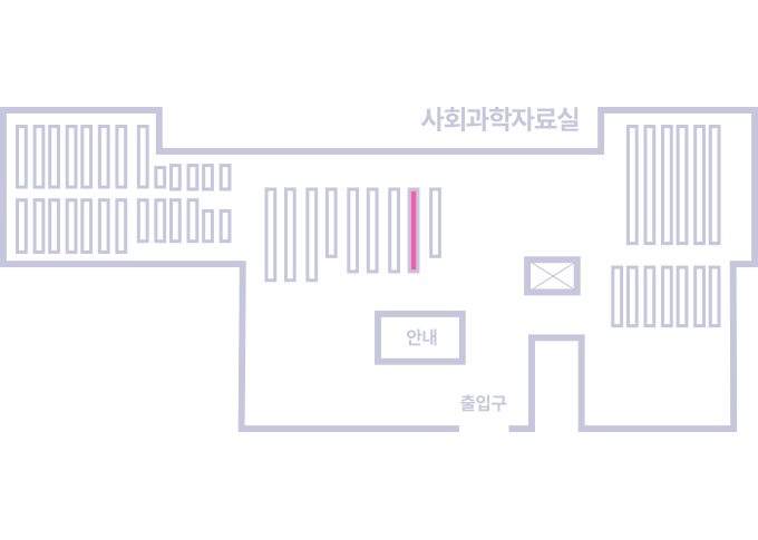
도서위치안내: / 서가번호:
우편복사 목록담기를 완료하였습니다.
*표시는 필수 입력사항입니다.
저장 되었습니다.