대표어
대표어


권호기사보기
| 기사명 | 저자명 | 페이지 | 원문 | 기사목차 |
|---|
결과 내 검색
동의어 포함
목차
[표제지]=0,1,1
제출문=i,2,1
보고서요약서=ii,3,1
요약문=iii,4,4
Summary=vii,8,4
Contents=xi,12,1
목차=xii,13,1
List Of Tables=xiii,14,1
List Of Figures=xiv,15,4
제1장 연구개발과제의 개요=1,19,2
제2장 국내외 기술개발 현황=3,21,2
제3장 연구개발 수행 내용 및 결과=5,23,1
제1절 역학과정=5,23,48
제2절 물리과정=53,71,1
1. 행성경계층 모수화 방안 개발=53,71,55
2. 예단 구름 미세물리과정 개발=108,126,37
3. 적운 모수화 방안 개발=145,163,77
4. 중력파 항력 모수화 방안 개발=222,240,28
5. 오존 역학 물리 과정 개발=250,268,29
6. 지면 모수화 방안 개발=279,297,6
제3절 자료동화=285,303,55
제4절 통합시스템 구축 및 검증=340,358,7
제4장 목표달성도 및 관련분야에의 기여도=347,365,2
제5장 연구개발결과의 활용계획=349,367,1
제6장 참고문헌=350,368,5
Fig.1.1. Time-Zonal Mean Of Zonal Velocity(Upper Row) And Temperature(Lower Row) Of 1200-Day HSW Simulation. Contour Intervals For The Velocity And Temperature Are 5㎳-1 And 10 K, Respectively, And Thick Contour For Zonal Flow Represents 30㎳-1=8,26,1
Fig.1.2. CPU Time Required For 10-Timestep Time Integration Of The DFS And SHM Dynamical Cores On The Supercomputer NEC SX-5(Parallel Vector Machine), Where A Single Processor(Theoretical Peak Performance : 10 GFLOPS) Was Used=9,27,1
Fig.2.2.1. Vertical Cross Section Of Precipitation(g ㎏-1) (Snow-Shaded; Rain-Lines) From NCEP Cloud 5. Sedimentation Of Falling Precipitation After(Left) And Before(Right) Updating Water Substance In The Cloud Scheme=109,127,1
Fig.2.2.2. (a) Satellite Imagery At 0000 UTC 25 June 1997, And The Corresponding 36-hr Forecasted Accumulated Cloud With (b) Modified Scheme And (c) Old Scheme=109,127,1
Fig.2.2.3. (a) Ice Number Concentration Distribution And (b) Ice Deposition Rate With Respect To Temperature=110,128,1
Fig.2.3.1. Time Series Of The Rainfall Amount(㎜ hr-1) Obtained From TOGA Data(Open Circle), CNTL(Gray), And SALL(Black) Experiments: (a) Total Rain, (b) Convective Rain, And (c) Precipitation Due To The Large-Scale Condensation=147,165,1
Fig.2.3.2. (a) Apparent Heat Sources(K day-1) And (b)Moisture Sinks(K day-1) Obtained From Cumulus Convections Of Each Experiment. Vertical Axis In (a) And (b)Denotes The Sigma Value With Surface Pressure Of 1005 hPa=148,166,1
Fig.2.3.3. Mean Precipitation(㎜ Month-1) Averaged For The Summers Of The 3 Years(1996, 1997, And 1999) For (a) The Observation And (b) The CNTL Run. Contour Intervals Are 200㎜, Except For That The First Contour Designates 100㎜=149,167,1
Fig.2.3.4. Same As In Fig.2.7 For (a),(b),(c),(d), And (e),(f),(g),(h) Their Differences (㎜ Month-1) From The CNTL Case. Contour Interval For The Precipitation Differences Is 100㎜, Staring From 50㎜. Zero Line Is Omitted. In The Right Panels=150,168,1
Fig.2.4.1. Schematic Diagram Of The Basic-State Wind And Stability. The Symbols Zb, Zt, And Zs Represent The Bottom And Top Heights Of The Diabatic Forcing And The Top Height Of Shear Layer, Respectively=223,241,1
Fig.2.4.2. (Top) The Basic-State Wind Profiles And(Bottom) The Analytic Wave Momentum Flux Spectra And Numerically Calculated Momentum Flux Spectra For (a) A Midlatitude Squall Line Simulated By Song et Al=226,244,1
Fig.2.4.3. (a) The Basic-State Wind Profiles, (b) Three-Dimensional Analytic Zonal Wave Momentum Flux Spectrum, And (c) Momentum Flux Spectrum Above A Tropical Convective System Simulated By Piani et al=226,244,1
Fig.2.4.4. Zonal Wind And Wave Momentum Forcing Calculated Using LM And WM Methods For (a) The Westerly And (b) The Easterly QBO Phases Considered In Piani et al. (2000)=229,247,1
Fig.2.4.5. Latitude-Height Cross Sections Of Zonally Averaged Zonal Wind And Zonal Wave Momentum Forcing Obtained Using LM(F2c=0.01) And WM(β=0.7) Methods In (a) January And (b) July=230,248,1
Fig.2.4.6. Time-Height Cross Sections Of Zonal-Mean Zonal Wind(Black Contour) And Zonal Wave Momentum Forcing(Shading) Averaged Over 15˚S-15˚N For (a) LM (F2e=0.01) And (b) WM (β=0.7)=231,249,1
Fig.2.5.1. Schematic Diagram Of SCM=251,269,1
Fig.2.5.2. Schematic Diagram Of Data Analysis System=252,270,1
Fig.2.5.3. Differences Of The (a) Temperature And (b) Relative Humidity Between Observation And SCM Results=255,273,1
Fig.2.5.4. Cloudiness From (a) Observation And (b) The SCM=256,274,1
Fig.2.5.5. Cloud Optical Thickness From The (a) SCM And (b) MODIS=257,275,1
Fig.2.5.6. Comparison Of The Ozone And Temperature Profiles Of SCM And Observation : (a) 4 March, (b) 18th March=258,276,1
Fig.2.5.7. (a) Downward And (b) Upward Long-Wave Radiation From Observation And The SCM=259,277,1
Fig.2.5.8. Same As Fig.2.5.7, But For Short-Wave Radiation=260,278,1
Fig.2.5.9. Comparison Of (a) Cloudiness Of The GOES Satellite And (b) The Observed Precipitable water With The SCM Results=261,279,1
Fig.2.5.10. Difference Profiles For (a) Ozone And (b) Temperature Between Experiment With Doubled Ozone And Control Run=262,280,1
Fig.2.5.11. Differences Of Heating Rate In (a) Short-Wave And (b) Long-Wave In SCM=263,281,1
Fig.2.5.12. Schematic Diagram Of The Comparison Between The SCM And Observation=263,281,1
Fig.3.1.1. Schematic Diagram Of GDAS Routines=288,306,1
Fig.3.1.2. Distribution Of Temperature Data. Data Subset Type, Number Of Data, And Data Type Index Are Shown On The Each Figure=291,309,1
Fig.3.1.3. Same As Fig.3.1.2 But For Specific Humidity=292,310,1
Fig.3.1.4. Same As Fig.3.1.2 But For Surface Pressure=292,310,1
Fig.3.1.5. Same As Fig.3.1.2 But For Satellite Temperature=293,311,1
Fig.3.1.6. Same As Fig.3.1.2 But For Wind=294,312,1
Fig.3.1.7. Same As Fig.3.1.2 But For Satellite Wind=295,313,1
Fig.3.1.8. 500 hPa Height Monthly Mean Difference(m) From The Control Run In Dec. 1997=300,318,1
Fig.3.1.9. Same As Fig.3.1.8, But For 850 hPa Temperature=301,319,1
Fig.3.1.10. Same As Fig.3.1.8, But For Precipitation=302,320,1
Fig.3.2.1. Schematic Diagram Of Local Ensemble Kalman Filter=336,354,1
Fig.3.2.2. Flow Chart Of Experiment Execution. The Name In Square Is The Name Of Subroutine Program In Each Process And Nlobs Means The Number Of Observation Data=337,355,1
Fig.3.2.3. Time Series(According To The Analysis Cycle) Of RMS Of Each Level Using The Local Ensemble Kalman Filter In Quasi-Geostropic Model. Analysis Variable Is Streamfunction, And Total Number Of Ensemble Is 25=338,356,1
Fig.4.1. Schematic Diagram Of YOURS GSM=341,359,1
Fig.4.2. Schematic Diagram Of The Unified System That Combines The KMA-GDAS And YOURS GDPAS=341,359,1
Fig.4.3. Anomaly Correlations Of (a) 850 hPa Temperature, (b) 500 hPa Temperature And (c) 500 hPa Geopotential Height Over Northern Hemisphere(Upper Penal) And Southern Hemisphere(Lower Penal) For 5-Day Forecast On 1200 UTC July 2001=342,360,1
Fig.4.4. Same As Fig.4.3, Except For RMSE=343,361,1
Fig.4.5. Same As Fig.4.4 Except For (a) 850 hPa U-Wind And (b) 250 hPa U-Wind=344,362,1
Fig.4.6. 14 July 2001 Daily Precipitation(㎜ day-1) From (a) GPCP, (b) KMA-T213 And (c) G62DA. Contour Interval Is 5㎜ day-1. Shading Designates The Precipitation Amount Greater Than 20 And 40㎜ day-1(이미지참조)=345,363,1
Fig.4.7. Monthly Precipitation(㎜/month) Of 4-Day Prediction From (a) GPCP, (b) KMA-T213 And (c) G62DA For July 2001=346,364,1
영문목차
[title page etc.]=0,1,3
Summary(In Korean)=iii,4,4
Summary=vii,8,4
Contents=xi,12,1
Contents(In Korean)=xii,13,1
List of Tables=xiii,14,1
List of Figures=xiv,15,4
Chapter1. Introduction=1,19,2
Chapter2. Current Status Of Technological Advances At Home And Abroad=3,21,2
Chapter3. Contents And Results Of R&D Execution Of Project=5,23,1
Section1. Dynamic System=5,23,48
Section2. Physical Processes=53,71,1
1. Vertical Diffusion Parameterization Scheme=53,71,55
2. Explicit Cloud Scheme=108,126,37
3. Convective Parameterization Scheme=145,163,77
4. Gravity Wave Drag Scheme=222,240,28
5. Radiation Physics=250,268,29
6. Land-Surface Processes=279,297,6
Section3. Data Assimilation=285,303,55
Section4. Development And Evaluation Of The Unified System=340,358,7
Chapter4. Achievement Of R&D Aims And External Contribution=347,365,2
Chapter5. Plans For Utilization Of R&D Results=349,367,1
Chapter6. References=350,368,5
*표시는 필수 입력사항입니다.
| 전화번호 |
|---|
| 기사명 | 저자명 | 페이지 | 원문 | 기사목차 |
|---|
| 번호 | 발행일자 | 권호명 | 제본정보 | 자료실 | 원문 | 신청 페이지 |
|---|
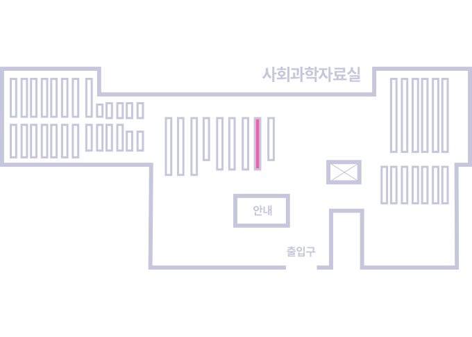
도서위치안내: / 서가번호:
우편복사 목록담기를 완료하였습니다.
*표시는 필수 입력사항입니다.
저장 되었습니다.