


권호기사보기
| 기사명 | 저자명 | 페이지 | 원문 | 기사목차 |
|---|
| 대표형(전거형, Authority) | 생물정보 | 이형(異形, Variant) | 소속 | 직위 | 직업 | 활동분야 | 주기 | 서지 | |
|---|---|---|---|---|---|---|---|---|---|
| 연구/단체명을 입력해주세요. | |||||||||
|
|
|
|
|
|
* 주제를 선택하시면 검색 상세로 이동합니다.
목차
[표제지]=0,1,1
제출문=1,2,1
보고서 요약서=2,3,1
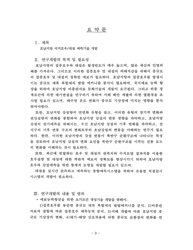
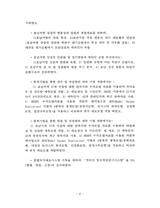
요약문=3,4,9
Summary=12,13,9
목차=21,22,4
Contents=25,26,4
List of Figures=29,30,11
List of Tables=40,41,5
제1장 서론=45,46,1
제1절 연구개발의 필요성=45,46,2
제2절 연구개발의 최종목표=46,47,1
제2장 국내ㆍ외 기술개발 현황=47,48,2
제3장 기술개발수행 내용 및 결과=49,50,1
제1절 집중호우를 동반한 MMC의 발달 메커니즘 분석=49,50,1
1. 서론=49,50,1
2. 기상현황 및 일기도 분석=50,51,6
3. 비종관 자료분석=55,56,6
4. 지형 강제력이 중규모 대류 복합체 발달에 미치는 영향 분석=61,62,4
5. 결론=64,65,2
제2절 비종관 자료의 결합에 따른 집중호우 예측능력 분석=66,67,1
1. 서론=66,67,2
2. 호남지방의 지형 및 기후특성=67,68,2
3. 호남지방 기상예측시스템과 LAPS 시스템=68,69,7
4. 관측자료 분석=74,75,6
5. 수치실험 설계=79,80,6
6. 레이더 자료동화 민감도 분석=84,85,11
7. 결론=94,95,2
제3절 서해 개펄에 따른 호남지방 중규모 기상장의 변화=96,97,1
1. 서론=96,97,1
2. 개펄의 현황 및 지형=96,97,3
3. 수치모형=99,100,1
4. 개펄의 열수지=99,100,3
5. 개펄의 노출에 따른 대기의 변화=102,103,3
6. 결론=104,105,2
제4절 대기-해양 상호작용에 의한 중규모 순환장의 변화=106,107,1
1. 서론=106,107,3
2. 이론적 배경=108,109,3
3. 수치모형=110,111,2
4. 제주도의 기상특징=111,112,4
5. 실험설계=114,115,7
6. 결과분석 - 마찰에 대한 소용돌이의 변화=121,122,7
7. 결과 분석 - 대기/해양의 해수면 상태에 따른 칼만와열의 변화=128,129,59
8. 결론=187,188,1
제5절 호남지방 강설의 변동성과 강설의 계절예보=188,189,1
1. 서론=188,189,2
2. 국내외 기술개발 현황=189,190,1
3. 연구개발 수행내용 및 결과=189,190,1
3.1. 한반도 및 호남지방 강설=189,190,15
3.2. 호남지방 강설과 북반구 대기순환 구조=204,205,20
3.3. 호남지방 강설의 장기예측=224,225,8
3.4. 요약 및 결론=231,232,3
제6절 호남지방 강설의 연변화 및 장기변동과 북반구 순환 특성=234,235,1
1. 서론=234,235,1
2. 국내외 기술개발 현황=235,236,1
3. 기술개발 내용 및 결과=236,237,1
3.1. 연구자료 및 분석방법=236,237,2
3.2. 호남지방 강설의 연변화=238,239,7
3.3. 호남지방 강설의 장주기 변화=245,246,11
3.4. 논의 및 결론=255,256,3
제7절 통계기법을 통한 강수 예측기법 개발=258,259,1
1. 서론=258,259,1
1.1. 개발의 목적과 필요성=258,259,1
1.2. 기상재해와 집중호후=258,259,3
2. 국내ㆍ외 기술개발 현황=260,261,3
3. 기술개발수행 내용 및 결과=262,263,1
3.1. 개발 내용=262,263,1
3.2. 개발에 사용된 자료=262,263,6
3.3. 예측량과 예측인자에 대한 탐색적 분석=268,269,5
3.4. 예측모델 개발 전략=273,274,3
3.5. 적용되는 통계 모형들=275,276,10
3.6. 강수량예측=284,285,20
3.7. 집중호우 발생 예측=303,304,28
3.8. 결론 및 요약=330,331,3
제8절 호남지역 강설예보를 위한 통계 모형 개발=333,334,1
1. 서론=333,334,1
2. 연구 범위=333,334,2
3. 개발에 사용된 자료=334,335,1
3.1. 예측량과 예측인자들=334,335,2
3.2. 군집분석=335,336,3
4. 예측모델 개발 전략=337,338,1
4.1. 예측 모형=337,338,3
4.2. 예측성 평가 측도=339,340,2
5. 강설량 예측=340,341,1
5.1. 중회귀모형=340,341,6
5.2. 신경회로망 모형=345,346,7
5.3. 결정나무 모형=351,352,7
5.4. 모형의 비교=357,358,2
6. 세범주 대설예보=358,359,1
6.1. 다등급 로지스틱 회귀모형=358,359,5
6.2. 신경회로망 모형=362,363,3
6.3. 결정나무 모형=364,365,3
6.4. 모형의 비교=366,367,2
7. 결론 및 요약=368,369,2
제9절 영상기반 적설 원격관측시스템의 설치=370,371,1
1. 설치 위치의 선정=370,371,2
2. 시스템의 규격=371,372,7
3. 시스템의 설치=377,378,2
제4장 연구개발 결과의 활용계획=379,380,1
참고문헌=380,381,9
Fig. 1.1. Synoptic Chart Of Surface From 18UTC To 03UTC 14 July 2004 With 3Hours Interval, Which Was Provided By Korea Meterological Administration=50,51,1
Fig. 1.2. Synoptic Chart Of 850hPa And 500hPa At 12UTC 14 July 2004 Which Were Provided By Korea Meterological Administration=51,52,1
Fig. 1.3. Temperature, Pressure,A And Wind Variation During MCC Passing In Jindo At Two Days From 13 July 2004=51,52,1
Fig. 1.4. Variation Of Precipitation Observed By Rain Gage From 04LST To 14LST 14 July 2004 With 2Hours Interval=52,53,1
Fig. 1.5. The Auxiliary Analysis Chart I(2004. 7. 14. 00UTC)=53,54,1
Fig. 1.6. The Auxiliary Analysis Chart II(2004. 7. 14. 00UTC)=54,55,1
Fig. 1.7. Div-Q Vector Values From (a)03, (b)06, And (C)09LST 14 July 2004. Dashed And Solid Lines Indicate Conversion And Diversions Area, Respectively=55,56,1
Fig. 1.8. Evolution Of MCCdetected By GEOS IR Sensor At 14 July 2004=56,57,1
Fig. 1.9. RHI Image Of Muan X Band Radar At 14 July 2004=57,58,1
Fig. 1.10. Time Variation Of Wind Vector Observed By Muan Doppler Radar Per Every 10Minute (2004. 7. 14. 01~44 KST)=58,59,1
Fig. 1.11. Hodo Graph Of Wind At 18 And 21 UTC 13, July In Heanam=58,59,1
Fig. 1.12. SRH Calculated By Data Of Heanam Site=59,60,1
Fig. 1.13. Skew-T Diagram Observed At Gwangju. The Observation Time Is a) 18LST 13 July, And b) 00LST 14 July 2004=60,61,1
Fig. 1.14. Topography Of Model Domains Used In This Study=62,63,1
Fig. 1.15. Location Of Elimination Area In Numerical Experiments. Rectangular Area Indicate Elimination Area At 34-35˚N And 125-125.7˚E=63,64,1
Fig. 1.16. Distribution Of Accumulated Precipitation By a) Simulation And b) Observation For Three Hours=63,64,1
Fig. 1.17. Distribution Of Accumulated Precipitation Simulated In a) Case 1 And b) Case 2=64,65,1
Fig. 2.1. The Flow Diagram Of LAPS Analysis Cycle=70,71,1
Fig. 2.2. The Flow Diagram Of LAPS Surface Analysis=71,72,1
Fig. 2.3. The Flow Diagram Of LAPS 3-D Wind Analysis(Albers, 1995)=71,72,1
Fig. 2.4. The Flow Diagram Of LAPS 3-D Temperature Analysis=72,73,1
Fig. 2.5. The Flow Diagram Of LAPS 3-D Moisture Analysis(Birkenheuer, 1992)=72,73,1
Fig. 2.6. The Flow Diagram Of LAPS 3-D Cloud Analysis(Albers, 1996)=73,74,1
Fig. 2.7. The Surface Weather Chart And GMS Image(Up)/Radar Image And AWS Precipitation(Down) At 00UTC 17 July 2003=75,76,1
Fig. 2.8. The Surface Weather Chart And GMS Image(Up)/Radar Image And AWS Precipitation(Down) At 00UTC 18 July 2003=76,77,1
Fig. 2.9. The Surface Weather Chart And GMS Image(Up)/Radar Image And AWS Precipitation(Down) At 00UTC 21 July 2003=76,77,1
Fig. 2.10. The Surface Weather Chart And GMS Image(Up)/Radar Image And AWS Precipitation(Down) At 00UTC 22 July 2003=77,78,1
Fig. 2.11. The Surface Weather Chart And GMS Image(Up)/Radar Image And AWS Precipitation(Down) At 00UTC 23 July 2003=77,78,1
Fig. 2.12. The Surface Weather Chart And GMS Image(Up)/Radar Image And AWS Precipitation(Down) At 00UTC 24 July 2003=78,79,1
Fig. 2.13. Wind Variation And Surface Precipitation At Gwangju For 10 Days From 14 July 2003=79,80,1
Fig. 2.14. The Model Domain And Their Topography Used In Regional Meteorological Prediction System. Horizontal Distance Of Grids Is 30 ㎞(Domain 1), 15㎞(Domain 2),And 5㎞(Domain 3), Respectively=80,81,1
Fig. 2.15. The Surface Weather Chart At 00UTC 22 July 2003 (Up) And 12UTC 22 July 2003(Down). Rectangle Means Target Area And Arrow Is Indicated The Movement Of Low Pressure=81,82,1
Fig. 2.16. The Same As Fig. 16 Except For 00UTC 23 July 2003 (Up) And 12UTC 23 July 2003(Down)=82,83,1
Fig. 2.17. Radar Echo Detected By Jindo S-Band Radar(Up) And AWS Precipitation(Down Left)/Doppler Velocity PPI Image(Down Right) At 22 July 2003=83,84,1
Fig. 2.18. Radar Echo Detected By Jin-Do S-Band Radar(Up) And AWS Precipitation (Down Left) / Doppler Velocity PPI Image(Down Right) At 23 July 2003=84,85,1
Fig. 2.19. Simulated Surface Wind Field Without Radar Assimilation Data At 00LST 22 July 2003=85,86,1
Fig. 2.20. Same As Fig. 2.19 Except For 12LST 22 July 2003=86,87,1
Fig. 2.21. Same As Fig. 2.19 Except For 00LST 23 July 2003=86,87,1
Fig. 2.22. Same As Fig. 2.19 Except For 12LST 23 July 2003=87,88,1
Fig. 2.23. Simulated Surface Wind Field With Radar Assimilation Data At 00LST 22 July 2003=88,89,1
Fig. 2.24. Same As Fig. 2.23Except For 12LST 22 July 2003=88,89,1
Fig. 2.25. Same As Fig. 2.23 Except For 00LST 23 July 2003=89,90,1
Fig. 2.26. Same As Fig. 2.23 Except For 121St 23 July 2003=89,90,1
Fig. 2.27. Simulated Surface Precipitation Without Radar Assimilation Data At 00LST 22 July 2003=90,91,1
Fig. 2.28. Same As Fig. 2.27 Except For With Radar Data Assimilation At 00LST 22 July 2003=91,92,1
Fig. 2.29. Simulated Surface Precipitation Without Radar Assimilation Data At 00LST 23 July 2003=91,92,1
Fig. 2.30. Same As Fig. 2.27 Except For With Radar Data Assimilation At 001St 23 July 2003=92,93,1
Fig. 2.31. Difference Of Precipitation Between With/Without Radar Data Assimilation At 22 July 2003=92,93,1
Fig. 2.32. Difference Of Precipitation Between With/Without Radar Data Assimilation At 23 July 2003=93,94,1
Fig. 3.1. Topography Of Model Domain And Locations Of Ebb Tide Observation=98,99,1
Fig. 3.2. Tidal Flat Distribution In Western Part Of Korean Peninsula. Blue Dashed Line Indicate Lower Tidal Flat Used In Numerical Simulation=98,99,1
Fig. 3.3. Observation Depths Of Sediment Temperature In The Tidal Flat And Photography Of Data Recorder=100,101,1
Fig. 3.4. Diurnal Variation Sediment Temperature, Wind, Solar Radiation, And Tidal Spectrum In Summer Season=101,102,1
Fig. 3.5. Surface Wind Vectors Simulated With Tidal Flat Variation At 1400LST=102,103,1
Fig. 3.6. Same As Fig.3.5 Except For Vectors Without Tidal Flat Variation=103,104,1
Fig. 3.7. Surface Wind Vectors Simulated With(Black Arrows) And Without(Pink Arrows) Tidal Flat Variation=104,105,1
Fig. 4.1. The MM5 Modeling System Flow Chart=111,112,1
Fig. 4.2. Location And Topography Of Jeju Island, Korea=113,114,1
Fig. 4.3. a)Wind Rose Of Monthly Average For 30 Years In Jeju And b) Vertical Wind Profile Observed At Gwangju 00UTC 13 December 2003=114,115,1
Fig. 4.4-1. The Model Domains And Their Terrains For This Study. Solid Line In b) Is Cross-Section Line For Vertical Analysis=117,118,1
Fig. 4.4-2. The Land Use Of Jeju Islands. 3 Is Irrg. Crop. Past, 6 Is Crop/Wood Mosaic, 8 Is Shrubland, 14 Is Everygreen Needlf, 15 Is Mixed Forest, 16 Is Water Bodies=118,119,1
Fig. 4.5. Infrared Image Detected By GEOS Satellite At 12 December 2003=120,121,1
Fig. 4.6. Synoptic Chart Of a) Surface, And b) 500hPa In 09LST 12 December 2003=120,121,1
Fig. 4.7. Stream Lines Distribution At 1㎞ Height Under Different Roughness Length After 42 Hours Integration. Upper, Middle, And Lower Panels Are In With Om, Lm ,And 5M Surface Roughness Length , Respectively=122,123,1
Fig. 4.8. Location Of Analysis And Topography Of The Hanla Mountain In Jeju Island=122,123,1
Fig. 4.9. Variation Of Wind Velocity At A, B, C, And D Of Fig.5. Colors Indicates Simulation Cases And Navy, Pink, And Yellow Line Mean Wind Velocity Which Were Calculated By Case LOW=124,125,1
Fig. 4.10. Variation Of Daily Mean Wind Velocity For The Period Of December 2002=125,126,1
Fig. 4.11. The Same As In Fig. 4.10, Except For The Period Of January 2003=125,126,1
Fig. 4.12-1. Time Series Of Streamlines At 900hPa Calulated By Case 1. The Times Are a)000LST, b)0300LST, c)0600LST, d)0900LST, e)1200LST, f)1500LST, g)1800LST, And h)2100LST=129,130,2
Fig. 4.12-2. Same As In Fig. 4.12-1 Except For Case2=131,132,2
Fig. 4.12-3. Same As Fig. 4.12-1 Except For Case3=133,134,2
Fig. 4.13-1. Time Series Of Vertical Cross Section Of Potential Vorticity And Wind Vector Calulated By Case 1 Along The A-A' Line Indicated At Fig.8=136,137,2
Fig. 4.13-2. Same As Fig. 4.13-1 Except For Case 2=138,139,2
Fig. 4.13-3. Same As Fig. 4.13-1 Except For Case 3=140,141,2
Fig. 4.14-1. Time Series Of Vertical Cross Section Of Potential Temperature Calculated By Case 1 Along The A -A' Line Indicated At Fig.8.=143,144,2
Fig. 4.14-2. Same As Fig. 4.14-1 Except For Case 2=145,146,2
Fig. 4.14-3. Same As Fig. 4.14-1 Except For Case 3=147,148,2
Fig. 4.15-1. Time Series Of Potential Vorticity(Pv) At 800hPa Which Was Calculated By Case1 : The Interval Is 5 Pv. Note: 1PVU=10 -6㎞²kg-¹s-¹=150,151,2
Fig. 4.15-2. Same As In Fig. 4.15-1 Except For 900 hPa=152,153,2
Fig. 4.15-3. Same As Fig. 4.15-1 Except For 1000 hPa=154,155,2
Fig. 4.15-4. Same As Fig. 4.15-1 Except For Case 2=156,157,2
Fig. 4.15-5. Same As Fig. 4.15-1 Except For Case 2 And 900 hPa=158,159,2
Fig. 4.15-6. Same As Fig. 4.15-1 Except For Case 2 And 1000 hPa=160,161,2
Fig. 4.15-7. Same As Fig. 4.15-1 Except For Case 3=162,163,2
Fig. 4.15-8. Same As Fig. 4.15-1 Except For Case 3 And 900 hPa=164,165,2
Fig. 4.15-9. Same As Fig. 4.15-1 Except For Case 3 And 900 hPa=166,167,2
Fig. 4.16-1. Time Series Of Divergence And Convergence At 800 hPa Which Was Calculated By Case1 : (+) Divergence, (-) Convergence=169,170,2
Fig. 4.16-2. Same As Fig. 4.16-1 Except For 900 hPa=171,172,2
Fig. 4.16-3. Same As Fig. 4.16-1 Except For 1000 hPa=173,174,2
Fig. 4.17-1. Time Series Of Cloud Distribution Which Was Calculated By Case1. The Times Are a)000LST, b)0300LST, c)0600LST, d)0900LST, e)1200LST, f)1500LST, g)1800LST, And h)21 00LST=175,176,2
Fig. 4.17-2. Same As In Fig. 4.17-1 Except For Case 2=177,178,2
Fig. 4.17-3. Same As In Fig. 4.17-1 Except For Case 3=179,180,2
Fig. 4.18-1. Time Series Of Precipitable Water Which Was Calculated By Case1. The Times Are a)000LST, b)0300LST, c)0600LST, d)0900LST, e)1200LST, f)1500LST, g)1800LST, And h)2100LST=181,182,2
Fig. 4.18-2. Same As Fig. 4.18-1 Except For Case 2=183,184,2
Fig. 4.18-3. Same As Fig. 4.18-1 Except For Case 3=185,186,2
Fig. 5.1. The Yearly Amount Of Snowfall And Yearly Number Of Snow Days (Upper Panel) And Their Annual Variances(Lower Panel)=190,191,1
Fig. 5.2. Annual Mean Amount Of Monthly Snowfall In Mm=191,192,1
Fig. 5.3. Annual Mean Number Of Monthly Snowfall Days=192,193,1
Fig. 5.4. First 6 Varimax Rotated Eofs Of The Yearly Amount Of Snowfall In Korea=193,194,1
Fig. 5.5. Number Of Snowfall Days In Each Range Of Snowfall Depth At The Specified Observation Station In Each Panel=195,196,1
Fig. 5.6. Interannual Variation Of Monthly Snowfall Depth In Mm At Observation Stations In Honam Area=198,199,1
Fig. 5.7. Interanual Variation Of Number Of Snowfall Days At Observation Stations In Honam Area=199,200,1
Fig. 5.8. Time Series Of Factor Loading Of Eigen Model In Honam Area On December, January And February (Upper Panel) And Mode 1 And 5 Over Korea(Lower Panel)=201,202,1
Fig. 5.9. Interannual Variation Of Mean Amount Of Snowfall And Total Number Of Snowfall Days Of Jeonju, Gwangju And Mogpo In December, January And February=202,203,1
Fig. 5.10. Interannual Variation Of Yearly Mean Snowfall Amount(Honam Snow Index) And Total Number Of Snowfall Days In Jeonju, Gwangju And Mogpo=203,204,1
Fig. 5.11. Seasonal Rank Correlation Between Honam Snow Index And Seasonal Mean Surface Pressure In The Northern Hemisphere=205,206,1
Fig. 5.12. Spring And Summer Composite Maps Of The Surface Pressure Anomaly To The Seasonal Normals For The 5 Highest Honam Snow Index(Left Panels) And The 5 Lowest Honam Snow Index (Right Panel)=206,207,1
Fig. 5.13. Same As In Fig. 5.12 Except For Autumn And Winter=207,208,1
Fig. 5.14. Same As In Fig. 5.11 Except For 850 hPa=208,209,1
Fig. 5.15. Same As In Fig. 5.11 Except For 700 hPa=209,210,1
Fig. 5.16. Same As In Fig. 5.11 Except For 500 hPa=209,210,1
Fig. 5.17. Same As In Fig. 5.11 Except For 300 hPa=210,211,1
Fig. 5.18. Same As In Fig. 5.12 Except For 500 hPa=211,212,1
Fig. 5.19. Same As In Fig. 5.12 Except For Autumn And Winter At 500 hPa Level=211,212,1
Fig. 5.20. Scatter Diagram Between Yearly Snowfall Amount And Monthly Snowfall Amount In Honam Area=213,214,1
Fig. 5.21. Rank Correlation Between One Month Snowfall Amount In Honam Area And Mean Surface Pressure(Left Panels) And Mean 500 hPa Geopotential Height(Right Panels) In December, January And February=214,215,1
Fig. 5.22. Rank Correlation Between June And October Mean Surface Pressure And December Snowfall Amount(Upper Panels)=215,216,1
Fig. 5.23. Same As In Fig. 5.22 Except For 500 hPa=216,217,1
Fig. 5.24. December, January And February Composite Maps Of The Surface Pressure Anomaly(Left Panels) And 500 hPa Geopotential Heights(Right Panels)=218,219,1
Fig. 5.25. Same As In Fig. 5.24 Except For The 5 Lowest Snowfall Amount Over Honam Area In Each Month=219,220,1
Fig. 5.26. Composite Maps Of June And October(Upper Panel), July And November (Middle Panel) And July And October(Lower Panel) Surface Pressure Anomaly To Each Month Normals=220,221,1
Fig. 5.27. Same As In Fig. 5.26 Except For 500 hPa=221,222,1
Fig. 5.28. Same As In Fig. 5.26 Except For 5 Years Of The Lowest Snowfall Amount Over Honam Area=222,223,1
Fig. 5.29. Same As In Fig. 526 Except For The 5 Years Of The Lowest Snowfall Amount Over Hoanm Area And At 500 hPa Level=223,224,1
Fig. 5.30. The Right Panels Is The Scatter Diagram With Quadratic Regression Lines Of The Annual Snowfall Amount Over Honam Area And Northern Hemisphere Circulation Index=225,226,1
Fig. 5.31. Time Series Of The Annual Snowfall Amount Over Honam Area (Solid Line) And Forecasted Value(Dashed Line) By The Equation(L) In Text Using The Spring 500 hPa Circulation Index=226,227,1
Fig. 5.32. Same As In Fig. 5.30 Except For December Snowfall Amount And May Surface Pressure And June 500 hPa Circulation Index=227,228,1
Fig. 5.33. Same As In Fig. 5.30 Except For January Snowfall Amount And August Circulation Index=228,229,1
Fig. 5.34. Same As In Fig. 5.30 Except For February Snowfall Amount And April Surface Pressure And August 500 hPa Circulation Index=228,229,1
Fig. 5.35. Same As In Fig. 5.31 Except For Monthly Snowfall Amount For December By Equation(2) Using June 500 hPa, January By Quation(3) Using 500 hPa And February By Equation(4)=231,232,1
Fig. 6.1. Annual Variations Of 10-Day Snowfall Amount(A) And Days(b) In Honam Area. The Vertical Bar Represents The Confidence Level Of 95% Of 10-Day Mean Value During Mid-November 1936 ~ Mid-March 2003=238,239,1
Fig. 6.2. Five Dominant Eigenvectors For The 10-Day Snowfall Amount In Honam Area=240,241,1
Fig. 6.3. Real Part Of Wavelet Coefficients For The Temporal Coefficients Of The Five Dominant Eigenvectors Of 10-Day Snowfall Amount In Honam Area. The Abscissa Is Time(Year) And The Ordinate Is Timescale=241,242,1
Fig. 6.4a. Distribution Of Correlation Coefficients Between The Temporal Coefficents Of 4 Leading Eigenvectors And Time Series Of 57 Winter Mean 500 hPa Geopotential Heights From December 1948 To February 2004=242,243,1
Fig. 6.4b. As In Fig. 6.4A Except For The Time Series Of 57 Autumn Mean 500 hPa Geopotential Heights From September 1948 To November 2003=243,244,1
Fig. 6.5. As In Fig. 6.3 Except For The Time Series Of Yearly, December, January And February Snowfall Amount In Honam Area. The Contour Interval Is 100㎜=246,247,1
Fig. 6.6. Global Wavelet Spectra Of The Time Series Of Yearly And Monthly Snowfall Amount Over Honam Area. The Abscissa Is Timescale(Year) And The Ordinate Is The Spectral Power Normalized By Total Variance=248,249,1
Fig. 6.7. Time Series Of The Anomalies In Mm Unit Due To The Dominant Cycles For The Yearly Snowfall Amount Over Honam Area=248,249,1
Fig. 6.8. As In Fig. 6.7 Except For The Dominant Cycles Over 20 Years Period For The Monthly Snowfall Amount=249,250,1
Fig. 6.9a. Distribution Of Correlation Coefficients Between The Time Series Of Anomalies Due To Dominant Cycles For Yearly Snowfall Amount In Honam Area=250,251,1
Fig. 6.9b. As In Fig. 6.9A Except For The Time Series Of 57 Autumn Mean 500 hPa Geopotential Heights From September 1948 To November 2003=251,252,1
Fig. 6.10. As In Fig. 6.9A Except For December Snowfall Amount Anomalies Due To Dominant Cycles Of 56-79 And 11-157 Years Period, January Snowfall Anomalies=252,253,1
Fig. 6.11a. The Winter Mean 500 hPa Geopotential Height Differences Normalized By The Standard Deviation Between The 15-Years Period Of A:1948.12-1963.3, B:1969.12-4984.2, C: 1989.12~2004.2=253,254,1
Fig. 6.11b. As In Fig. 6.11A Except For December, January And February=254,255,1
Fig. 7.1. Economic And Insured Losses With Trends=259,260,1
Fig. 7.2. Yearly Economic Losses=260,261,1
Fig. 7.3. Accumulated Amount Of Property Damage For Each Type (1993-2002)=260,261,1
Fig. 7.4. Stations=264,265,1
Fig. 7.5. Dendrogram During Warm Season In Honam Area=265,266,1
Fig. 7.6. Results Of Cluster Analysis (Warm Season In Honam Area)=265,266,1
Fig. 7.7. Results Of Cluster Analysis (Cold Season In Honam Area)=266,267,1
Fig. 7.8. Histogram Of Rainfall Amount (Total Case)=268,269,1
Fig. 7.9. Histogram Of Rainfall Amount (Rainy Case)=268,269,1
Fig. 7.10. Distributions Of Predictors=270,271,2
Fig. 7.11. Scatter Diagrams=272,273,1
Fig. 7.12. Shape Of Logistic Function=276,277,1
Fig. 7.13. Structure Of Neural Networks=278,279,1
Fig. 7.14. Example Of Decision Tree=281,282,1
Fig. 7.15. Comparison Of Roc Curves=282,283,1
Fig. 7.16. Scatter Plot Of Observed Value And Fitted Value Using Training Data=285,286,1
Fig. 7.17. Scatter Plot Of Observed Value And Fitted Value Using Validation Data=286,287,1
Fig. 7.18. Scatter Plot Of Observed Value And Fitted Value Using Training Data=289,290,1
Fig. 7.19. Scatter Plot Of Observed Value And Fitted Value Using Validation Data=289,290,1
Fig. 7.20. Structure Of Applied Neural Networks=293,294,1
Fig. 7.21. Scatter Plot Of Observed Value And Fitted Value Using Training Data=294,295,1
Fig. 7.22. Scatter Plot Of Observed Value And Fitted Value Using Validation Data=294,295,1
Fig. 7.23. Final Decision Tree=297,298,1
Fig. 7.24. Scatter Plot Of Observed Value And Fitted Value Using Training Data=298,299,1
Fig. 7.25. Scatter Plot Of Observed Value And Fitted Value Using Validation Data=298,299,1
Fig. 7.26. Distribution Of Estimated Probability Of Occurrence Of Heavy Rain=304,305,1
Fig. 7.27. Roc Curve Generated From Logistic Regression Estimates=305,306,1
Fig. 7.28. Distribution Of Estimated Probability In Logistic Regression With Main Effects And Interaction Effects=310,311,1
Fig. 7.29. ROC Curve Generated From Logistic Regression Estimates=311,312,1
Fig. 7.30. ROC Curves=316,317,1
Fig. 7.31. AIC=316,317,1
Fig. 7.32. Structure Of Applied Neural Networks=316,317,1
Fig. 7.33. Distribution Of Estimated Probability In Neural Networks=317,318,1
Fig. 7.34. ROC Curve Generated From Neural Networks=318,319,1
Fig. 7.35. Final Decision Tree=323,324,1
Fig. 7.36. Distribution Of Estimated Probability In Decision Tree=323,324,1
Fig. 7.37. ROC Curve Generated From Decision Tree=324,325,1
Fig. 7.38. ROC Curves=329,330,1
Fig. 8.1. Dendrogram=336,337,1
Fig. 8.2. Result Of Cluster Analysis=337,338,1
Fig. 8.3. Generation Of Forecasts Using Thresholds=339,340,1
Fig. 8.4. Scatter Plot Of Observed Value And Fitted Value Using Training Data (With First Order Interaction)=344,345,1
Fig. 8.5. Scatter Plot Of Observed Value And Fitted Value Using Validation Data (With First Order Interaction)=345,346,1
Fig. 8.6. Structure Of Applied Neural Networks=346,347,1
Fig. 8.7. Scatter Plot Of Observed Value And Fitted Value Using Training Data (Neural Networks)=348,349,1
Fig. 8.8. Scatter Plot Of Observed Value And Fitted Value Using Validation Data (Neural Networks)=348,349,1
Fig. 8.9. Scatter Plot Of Observed Value And Fitted Value Using Training Data (With First Order Interaction)=350,351,1
Fig. 8.10. Scatter Plot Of Observed Value And Fitted Value Using Validation Data (With First Order Interaction)=351,352,1
Fig. 8.11. Average Squared Error Plot (Without First Order Interaction)=352,353,1
Fig. 8.12. Final Decision Tree (Without First Order Interaction)=353,354,1
Fig. 8.13. Scatter Plot Of Observed Value And Fitted Value Using Training Data (Without First Order Interaction)=353,354,1
Fig. 8.14. Scatter Plot Of Observed Value And Fitted Value Using Validation Data(Without First Order Interaction)=354,355,1
Fig. 8.15. Average Squared Error Plot (With First Order Interaction)=355,356,1
Fig. 8.16. Final Decision Tree (With First Order Interaction)=355,356,1
Fig. 8.17. Scatter Plot Of Observed Value And Fitted Value Using Training Data (Without First Order Interaction)=356,357,1
Fig. 8.18. Scatter Plot Of Observed Value And Fitted Value Using Validation Data(Without First Order Interaction)=357,358,1
Fig. 8.19. Time Series Plot Of Observations And Forecasts In Jung-Ub=361,362,2
Fig. 8.20. Final Tree=365,366,1
Fig. 9.1. Distribution Of Annual Mean Snowfall Amounts In Korea=370,371,1
Fig. 9.2. Observation Sites(Hampyeong, Younggwang, And .Gochancg)=377,378,1
Fig. 9.3. Computer H/W And S/W=378,379,1
영문목차
[title page etc.]=0,1,3
Summary(Korean)=3,4,9
Summary=12,13,9
Contents(Korean)=21,22,4
Contents=25,26,4
List Of Figures=29,30,11
List Of Tables=40,41,5
Chapter 1. Introduction=45,46,1
Session 1. Necessity Of R&D=45,46,2
Session 2. Scope And Contents Of R&D=46,47,1
Chapter 2. State Of Domestic And International R&D=47,48,2
Chapter 3. Results Of R&D=49,50,1
Session 1. Analysis Of Mesoscale Convective Complex(MCC) Development With Heavy Rainfall=49,50,1
1. Introduction=49,50,1
2. Analysis Of Synoptic Condition=50,51,6
3. Analysis Of Non-Routine Data(Focus On Radar)=55,56,6
4. Influence Of Orographic Forcing On MCC Development=61,62,4
5. Conclusion=64,65,2
Session 2. Study On Non-Routine Data For Prediction Possibility Of Heavy Rainfall=66,67,1
1. Introduction=66,67,2
2. Topography And Characteristics Of Climate In Honam Districts=67,68,2
3. Moodung Short Weather Prediction System(MSWP) And Local Analysis And Prediction System(LAPS)=68,69,7
4. Analysis Of Observation Data=74,75,6
5. Design Of Numerical Experiment=79,80,6
6. Sensitivity Of Radar Data Assimilation On Heavy Rainfall=84,85,11
7. Conclusion=94,95,2
Session 3. Variation Of Mesoscale Meteorological Field On Mud Flats In Yellow Sea=96,97,1
1. Introduction=96,97,1
2. Topography And Status Of Mud Flats=96,97,3
3. Numerical Model=99,100,1
4. Heat Budget On Mud Flats=99,100,3
5. Interaction Between Atmosphere And Surface Of Mud Flats=102,103,3
6. Conclusion=104,105,2
Session 4. A Study On The Influence Of Atmosphere And Sea Surface On Mesoscale Circulations=106,107,1
1. Introduction=106,107,3
2. Theoretical Background=108,109,3
3. Numerical Model=110,111,2
4. Meteorological Characteristics Of Jeju Island=111,112,4
5. Design Of Numerical Experiments=114,115,7
6. Result - The Variation Of Vortex Depending On Friction=121,122,7
7. Result- The Evolution Of Kaman Vortex By Atmosphere And Sea Surface Interaction=128,129,59
8. Conclusion=187,188,1
Session 5. Interannual Variation And Seasonal Forecasting Of The Snowfalls Over Honam Arca In The Korean Peninsula=188,189,1
1. Introduction=188,189,2
2. Currents Status On The Domestic And Abroad Research=189,190,1
3. Contents And Results Of The Projects=189,190,1
3.1. Snowfall Characteristics Of The Korean Peninsula And Honam Area=189,190,15
3.2. Northern Hemisphere Circulation Patterns Associated With The Honam Area Snowfall=204,205,20
3.3. Long Range Forecasting Of Honam Snowfalls=224,225,8
3.4. Summary And Conclusions=231,232,3
Session 6. Annual And Interannual-Interdecadal Variations Of The Snowfall Over Honam Area And Its Associated Northern Hemisphere Circulations=234,235,1
1. Introduction=234,235,1
2. Current Status On The Domestic And Abroad Research=235,236,1
3. Contents And Results Of The Projects=236,237,1
3.1. Data And Analysis Procedures=236,237,2
3.2. Annual Variation Of Snowfall Amount In Honam Area=238,239,7
3.3. Interannual-Interdecadal Variations Of Snowfall Amount=245,246,11
3.4. Summary And Conclusions=255,256,3
Session 7. Development Of Statistical Models For The Prediction Of Rainfall In Honam Area=258,259,1
1. Introduction=258,259,1
1.1. Objectives And Needs Of Research=258,259,1
1.2. Weather Disasters And Heavy Rain=258,259,3
2. Current Status Of Technological Advances=260,261,3
3. Range Of Research And Results=262,263,1
3.1. Range Of Research=262,263,1
3.2. Data Used For Our Research=262,263,6
3.3. Analysis Of Potential Predictors And Predictand=268,269,5
3.4. Strategy Of Development Of Forecast Models=273,274,3
3.5. Statistical Models=275,276,10
3.6. Quantitative Precipitation Forecast=284,285,20
3.7. Occurrence Of Heavy Rain=303,304,28
3.8. Conclusions And Summary=330,331,3
Session 8. Development Of Statistical Models For The Prediction Of Snowfall In Honam Area=333,334,1
1. Introduction=333,334,1
2. Range Of Research=333,334,2
3. Data Used For Our Research=334,335,1
3.1. Predictand And Predictors=334,335,2
3.2. Cluster Analysis=335,336,3
4. Strategy Of Development Of Forecast Models=337,338,1
4.1. Forecast Models=337,338,3
4.2. Skill Score=339,340,2
5. Quantitative Forecast Of Snowfall=340,341,1
5.1. Multiple Regression Model=340,341,6
5.2. Neural Network Model=345,346,7
5.3. Decision Tree Model=351,352,7
5.4. Comparison Of Models=357,358,2
6. Ternary Occurrence Of Heavy Snow=358,359,1
6.1. Multigrade Logistic Regression Model=358,359,5
6.2. Neural Network Model=362,363,3
6.3. Decision Tree Model=364,365,3
6.4. Comparison Of Models=366,367,2
7. Conclusions And Summary=368,369,2
Session 9. SOSIRI(Snowing Observation System Used Infra-Red Image) Install=370,371,1
1. The Selection Of The Observation Location=370,371,2
2. The Specifications Of The Observation System=371,372,7
3. The Install Of The Observation System=377,378,2
Chapter 4. Feature Applications And Expected Effects=379,380,1
References=380,381,9
jpg
Fig. 5.5. Number Of Snowfall Days In Each Range Of Snowfall Depth At The Specified Observation Station In Each Panel=195,196,1
Fig. 5.6. Interannual Variation Of Monthly Snowfall Depth In Mm At Observation Stations In Honam Area=198,199,1
Fig. 5.7. Interanual Variation Of Number Of Snowfall Days At Observation Stations In Honam Area=199,200,1
Fig. 7.1. Economic And Insured Losses With Trends=259,260,1
*표시는 필수 입력사항입니다.
| 전화번호 |
|---|
| 기사명 | 저자명 | 페이지 | 원문 | 기사목차 |
|---|
| 번호 | 발행일자 | 권호명 | 제본정보 | 자료실 | 원문 | 신청 페이지 |
|---|
도서위치안내: / 서가번호:

우편복사 목록담기를 완료하였습니다.
*표시는 필수 입력사항입니다.
저장 되었습니다.
