대표어





권호기사보기
| 기사명 | 저자명 | 페이지 | 원문 | 기사목차 |
|---|
결과 내 검색
동의어 포함
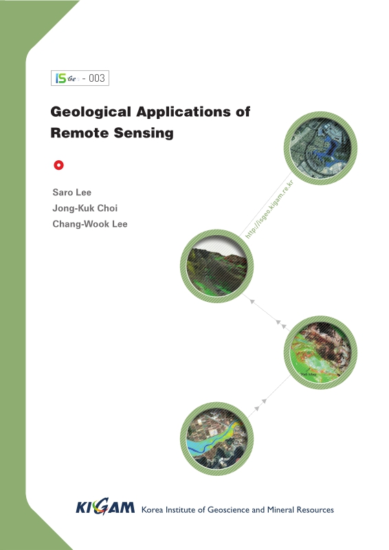
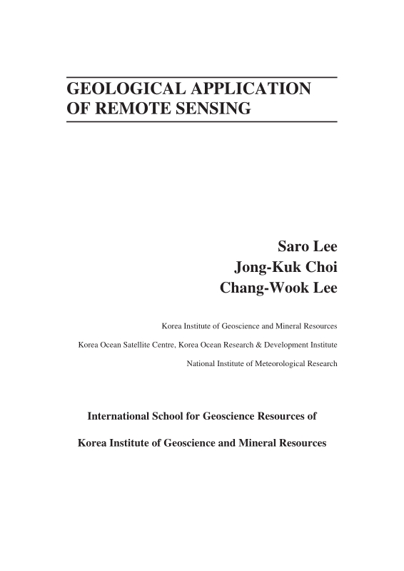
Title Page
[저자약력]
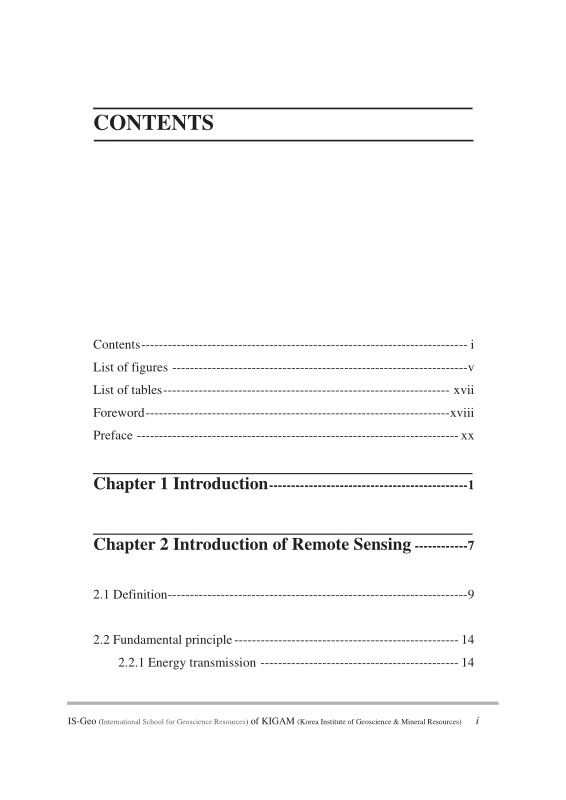
Contents
FOREWORD / Kyu Han Kim 22
PREFACE / Saro Lee ; Jongkuk Choi ; Chang-Wook Lee 24
Chapter 1. INTRODUCTION 26
Chapter 2. INTRODUCTION OF REMOTE SENSING 32
2.1. Definition 34
2.2. Fundamental principle 39
2.2.1. Energy transmission 39
2.2.2. Digital imaging and resolution 48
2.2.3. Spectral signature 55
2.3. Remote sensing system and image 62
2.3.1. Optical/Infrared remote sensing system 62
2.3.2. Microwave remote sensing system 65
2.3.3. Korean remote sensing system 66
2.4. Introduction of SAR 68
2.5. Introduction of hyperspectral remote sensing 71
Chapter 3. IMAGE PROCESSING OF REMOTE SENSING DATA 76
3.1. Introduction 78
3.2. Image restoration 79
3.3. Geometric correction 82
3.4. Image enhancement 88
3.5. Image composition 91
3.6. Special trnasformation; Principa Component Anaysis(PCA) and Vegetaion indices(VI) 95
3.6.1. Principal Component Analysis (PCA) 95
3.6.2. Vegetation Indices (VI) 100
3.7. Image classification 106
Chapter 4. GEOLOGICAL APPLICATION OF REMOTE SENSING 112
4.1. Geology 114
4.1.1. Geological structure 114
4.1.2. Lithology and mineral 120
4.2. Geological hazard 131
4.2.1. Land subsidence 131
4.2.2. Simulation of surface deformation 136
4.2.3. Volcano eruption monitoring 145
4.3. Ecology and ocean 160
4.3.1. Extraction of tidal information for habitat mapping 160
4.3.2. Mapping the temporal dynamics of coastal water turbidity using remote sensing 175
4.3.3. Application of the Geostationary Ocean Color Imager (GOCI) to estimates of ocean surface currents 195
Chapter 5. SUMMARY 212
Chapter 6. REFERENCES 216
Back Cover 240
Figure 2-1. Concept of remote sensing 34
Figure 2-2. Remote sensing studies in the Earth 35
Figure 2-3. Airborne remote sensing image of KIGAM(left) and space-borne remote sensing image of Seoul(right) 36
Figure 2-4. Active system and an optical image(left) and active system and a microwave image(right) 38
Figure 2-5. Electromagnetic wave 40
Figure 2-6. Long wavelength and short wavelength 41
Figure 2-7. Electromagnetic spectrum 42
Figure 2-8. Refraction and atmospheric scattering 43
Figure 2-9. Rayleigh scattering characteristics 44
Figure 2-10. Absorption of the Sun's incident electromagnetic energy in the region from 0.1 to 30 μm by various atmospheric gases 46
Figure 2-11. Various type of reflector 47
Figure 2-12. Combines effects of atmospheric absorption, scattering, and reflectance 48
Figure 2-13. Digital frame camera area array 49
Figure 2-14. Across-track or scanning mirror and single discrete detectors (whiskbroom) type 49
Figure 2-15. Linear array ("pushbroom", Along-track) type 50
Figure 2-16. Concept of digital image (=grid system). 51
Figure 2-17. Three method of display 52
Figure 2-18. Spatial resolutions 53
Figure 2-19. Spectral resolution 54
Figure 2-20. Temporal resolutions of MISR and MODI which are both on the TERRA satellite. 55
Figure 2-21. Spectral signatures of water, soil and vegetation (A) and a hypothetical example of how the LANDSAT satellite might record water, green... 56
Figure 2-22. Analytical Spectral Devices (ASD) is widely used field spectrometer 58
Figure 2-23. Including of Analytical Spectral Devices (ASD) 59
Figure 2-24. Measuring, processing and results of the reflectance of the target using ASD 60
Figure 2-25. Measuring optical properties of the surface water in the ocean using ASD 60
Figure 2-26. NOAA-AVHRR (left) and Landsat 7 ETM+(right) image 63
Figure 2-27. Image of the Burj Tower of Dubai, observed by KOMPSAT-3 in the fall of 2012(left) and SAR image of KOMPSAT/Arirang-5 of Sydney, Australia... 67
Figure 2-28. Airborne hyperspectral surveys using 200+ spectral channels from 0.38 to 2.5mm 71
Figure 2-29. Hyperion hyperspectral products from The EO-1 extended mission(NASA) 73
Figure 2-30. 3D mineral map for primary and secondary ore mineralization and alteration by airborne hyperspectral data 74
Figure 2-31. Hyperion instrument aboard EO-1 for geologic field detection(NASA) 75
Figure 3-1. Image processing in remote sensing. 79
Figure 3-2. Atmospheric effect 80
Figure 3-3. Image-to-map method of geometric correction 82
Figure 3-4. Acquiring GCPs in the field 83
Figure 3-5. Geocoding wizard of ER-mapper software for geometric correction of a raw image 84
Figure 3-6. Environmental setup 84
Figure 3-7. Selecting GCP and save the lists 85
Figure 3-8. Perspective projection(left) and polar stereo projection(right) 86
Figure 3-9. Transverse Mercator (TM) projection 86
Figure 3-10. Mosaic each single image into an integrated image 87
Figure 3-11. Image reduction and magnification 88
Figure 3-12. Contrast enhancement 89
Figure 3-13. Left images are the original image and the histogram. Right images are histogram enhanced image and its histogram 90
Figure 3-14. Colour composite images of Landsat 92
Figure 3-15. Image compositions for mineral exploration 92
Figure 3-16. Image pan-sharpening with QuickBird images. 93
Figure 3-17. Extracting tidal channel from pan-sharpened image. 94
Figure 3-18. Correlation matrix among seven Landsat TM bands of Charleston, SC 97
Figure 3-19. Diagrammatic representation of the spatial relationship between the first two principal components 98
Figure 3-20. PCA result for Landsat TM data of Charleston, S.C. obtained on Nov. 9, 1982 99
Figure 3-21. Principal component images for Landsat TM data of Charleston, S.C. obtained on Nov. 9, 1982 100
Figure 3-22. Absorption spectra of chlorophyll a and b 101
Figure 3-23. Typical spectral reflectance characteristics for healthy green grass, dead grass and bare dry soil 102
Figure 3-24. NDVI image of Yeoja Bay tidal flat 103
Figure 3-25. TVI image of Yeoja Bay tidal flat 104
Figure 3-26. MODIS EVI image – degree of green color indicates the biomass 105
Figure 3-27. Supervised classification 107
Figure 3-28. Assign the class to unknown pixel 107
Figure 3-29. Result image of supervised classification 109
Figure 3-30. Unsupervised classification 110
Figure 3-31. Unsupervised classification and determination of the ground cover for each of the clusters 111
Figure 4-1. Landsat spectral band information of seven different bands 115
Figure 4-2. Landsat band combinations with individual seven different bands 116
Figure 4-3. Landsat TM ratio image for geological structure 117
Figure 4-4. Geological structure image 118
Figure 4-5. Combination of Landsat TM ration image and SIR C/X image for interpretation of geological structure 119
Figure 4-6. A case study on the region, Mongolia 126
Figure 4-7. Case study area in Mongolia 126
Figure 4-8. Left is atmospherically uncorrected radiance-at-sensor data of ASTER Level 3A without cloud VNIR(RGB:Band 3, 2, 1) and right is... 127
Figure 4-9. Spectral emissivity curve of Carbonate rock, Quartz, Granite, Diorite, Gabbro and Peridotite 128
Figure 4-10. Left up is VNIR image, left down is RGB image, right down is geological map(1:200,000) and right up is projection image that projects VNIR... 129
Figure 4-11. (a) is VNIR image, (b) is quartz index map, (c) is SO₂ content index map, (d) is Carbonate index map, (e) is geological map, and (f) is... 129
Figure 4-12. Upper figure is IKONOS Image and bottom figure is Aerial photograph of reclaimed coastal land. Red squares represent 38 ground... 132
Figure 4-13. Generation seven good quality images and ten low quality images using eight SAR images from 9/15/02 to 10/28/03 133
Figure 4-14. High quality and low quality interferograms 134
Figure 4-15. Figure (A) shows in situ data by magnetic probe extensometers and Figure (B) represents DInSAR measurements. Figure (C), (D) and (E) show... 135
Figure 4-16. Two examples of (a, g) simulated deformation-only interferograms, (b, h) simulated topographic residual errors of interferograms, (c, i) simulated... 141
Figure 4-17. Simulation of surface deformation on the Seguam Volcano by using Mogi model from June 1993 to July 2007 142
Figure 4-18. Mean LOS velocity map from simulated deformation interferograms between June 1993 and July 2007. (b) Mean LOS velocity map derived from... 143
Figure 4-19. Simulated and SBAS-retrieved LOS time-series deformation at two locations. Crosses represent simulated time-series deformations, and circles show... 144
Figure 4-20. Location of Augustine Island in the southwestern part of Cook Inlet, Alaska 146
Figure 4-21. Geologic map showing the distribution of deposits from recent Augustine Volcano eruptions. Pyroclastic flow deposits emplaced in 1986 are... 147
Figure 4-22. Interferograms from European Remote Sensing Satellite (ERS)-1 and -2, and Environment Satellite (ENVISAT) Synthetic Aperture Radar (SAR)... 150
Figure 4-23. Observed high-coherence interferograms from track 229 ERS-1, ERS-2, and ENVISAT pairs. Each fringe (full color cycle) represents 28.3... 151
Figure 4-24. Averaged InSAR image from 229 tracks created by stacking all the unwrapped 1-year interferograms between 1992 and 2005 152
Figure 4-25. Perpendicular baselines used for small baseline subset(SBAS) interferometric synthetic aperture radar (InSAR) processing at Augustine volcano 154
Figure 4-26. Removal several error effects through SBAS processing. 155
Figure 4-27. Averaging deformation rate map for Augustine Volcano from the refined small baseline subset (SBAS) technique for the period 1992–2005. 156
Figure 4-28. Surface-displacement time-series for selected points on Augustine Volcano for the period 1992–2005. 157
Figure 4-29. (a) The Landsat ETM+ image of the Cheonsu Bay and Hwangdo tidal flat acquired on February 14, 2002. (b) The IKONOS RGB (432 bands)... 165
Figure 4-30. Control factors constructed in this case study. 173
Figure 4-31. (a) Bathymetric map of the case study area overlaid with the sampling stations in March and October 2011. (b) Mosaic of Landsat ETM+... 179
Figure 4-32. (a) RGB composite (R:680 nm, G:555 nm, B:412 nm) after Rayleigh reflectance correction generated from the GOCI image acquired at 12:30 local... 185
Figure 4-33. Match-up comparison of Rrs (660) between GOCI and in situ measurements using the 12 samples acquired on 26 October 2011. GOCI-derived... 186
Figure 4-34. SS algorithm used in the present case study, derived empirically from 34 observations of optical properties and SSC in March and October 2011 188
Figure 4-35. Map of SSC generated by GOCI band 5 based on the SS algorithm in Equation 1. 190
Figure 4-36. Relationship between in situ SSC (g/m3) and SSC (g/m3) derived from reflectance using the GOCI band centered at 660nm using the 12 samples... 191
Figure 4-37. Hourly variation in SSC at locations V1–V9 in Figure 4-32a 192
Figure 4-38. Color scenes derived from the GOCI. 199
Figure 4-39. Ocean colors derived from GOCI. 201
Figure 4-40. (a) A schematic diagram for estimating an ocean surface current vector. This methodology requires two data inputs: a source scene (S) (e.g.,... 203
Figure 4-41. A comparison between the trajectories of ocean surface current results (i.e., arrows) around coastal regions of Gyeonggi Bay using TSM scenes... 205
Figure 4-42. Comparisons between each ocean surface current vector results (i.e., directions (a) and velocities (b)) and in situ data obtained from Gyeonggi Bay on... 206
Figure 4-43. Daily SST data (i.e., colored image) provided by the GHRSST and the trajectories of the estimated ocean surface currents (i.e., arrows) from multiple... 208
| 등록번호 | 청구기호 | 권별정보 | 자료실 | 이용여부 |
|---|---|---|---|---|
| EM0000050547 | ER 전자형태로만 열람 가능함 | 이용가능 |
*표시는 필수 입력사항입니다.
| 전화번호 |
|---|
| 기사명 | 저자명 | 페이지 | 원문 | 기사목차 |
|---|
| 번호 | 발행일자 | 권호명 | 제본정보 | 자료실 | 원문 | 신청 페이지 |
|---|
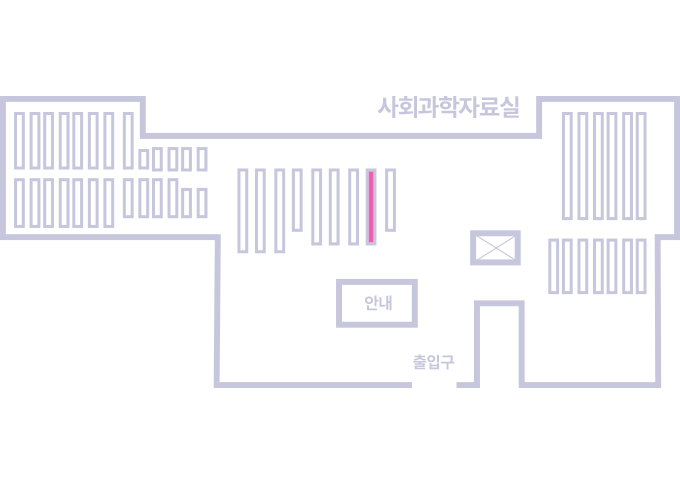
도서위치안내: / 서가번호:
우편복사 목록담기를 완료하였습니다.
*표시는 필수 입력사항입니다.
저장 되었습니다.