대표어

권호기사보기
| 기사명 | 저자명 | 페이지 | 원문 | 기사목차 |
|---|
결과 내 검색
동의어 포함
[표지]
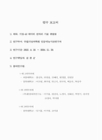
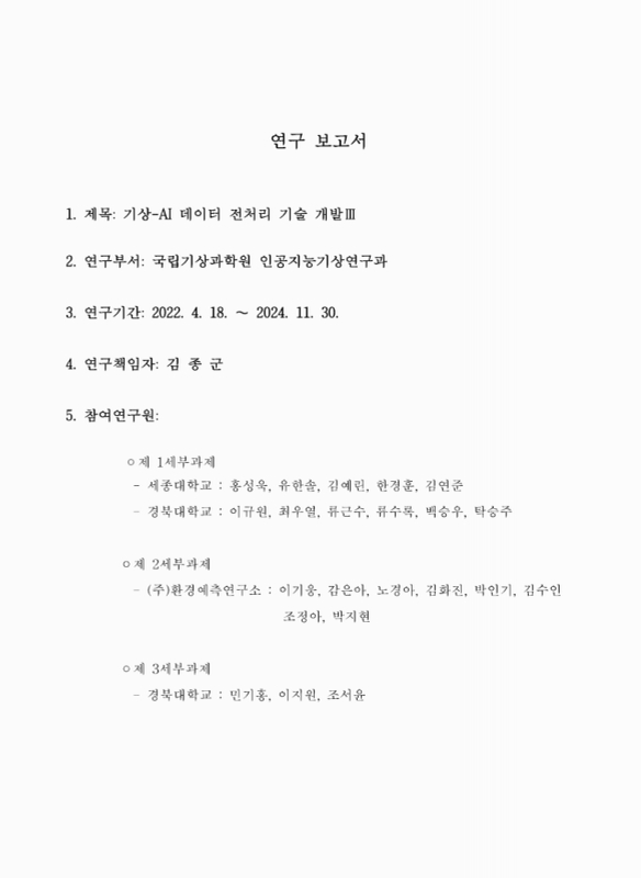
연구 보고서
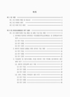
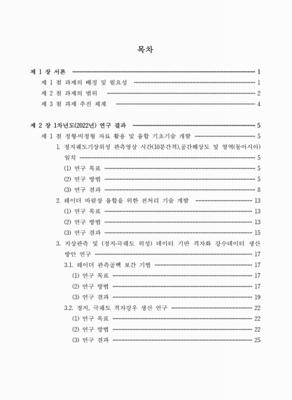
목차
요약문 27
제1장 서론 29
제1절 과제의 배경 및 필요성 29
제2절 과제의 범위 30
제3절 과제 추진 체계 32
제2장 1차년도(2022년) 연구결과 33
제1절 정형·비정형 자료 활용 및 융합 기초기술 개발 33
1. 정지궤도기상위성 관측영상 시간(10분간격), 공간해상도 및 영역(동아시아) 일치 33
2. 레이더 바람장 융합을 위한 전처리 기술 개발 41
3. 지상관측 및(정지·극궤도 위성) 데이터 기반 격자화 강수데이터 생산 방안 연구 45
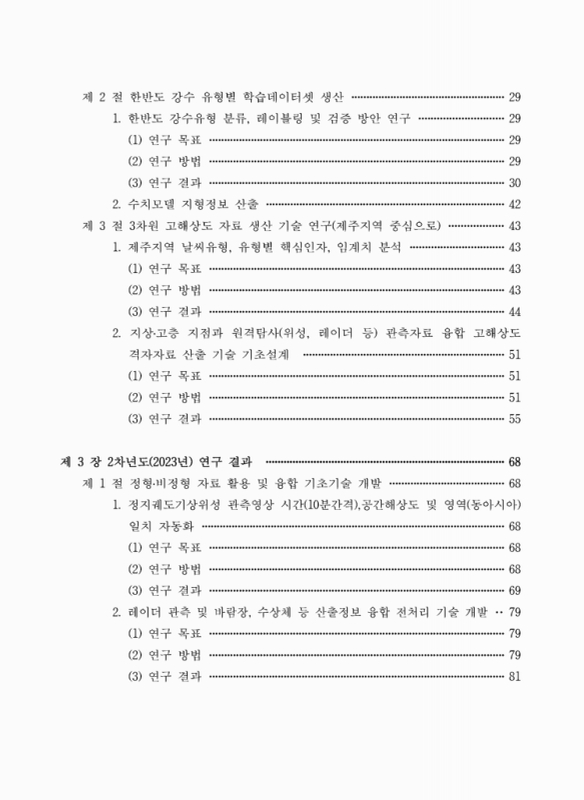
제2절 한반도 강수 유형별 학습데이터셋 생산 57
1. 한반도 강수유형 분류, 레이블링 및 검증 방안 연구 57
2. 수치모델 지형정보 산출 70
제3절 3차원 고해상도 자료 생산 기술 연구(제주지역 중심으로) 71
1. 제주지역 날씨유형, 유형별 핵심인자, 임계치 분석 71
2. 지상·고층 지점과 원격탐사(위성, 레이더 등) 관측자료 융합 고해상도 격자자료 산출 기술 기초설계 79
제3장 2차년도(2023년) 연구결과 96
제1절 정형·비정형 자료 활용 및 융합 기초기술 개발 96
1. 정지궤도기상위성 관측영상 시간(10분간격), 공간해상도 및 영역(동아시아) 일치 자동화 96
2. 레이더 관측 및 바람장, 수상체 등 산출정보 융합 전처리 기술 개발 107
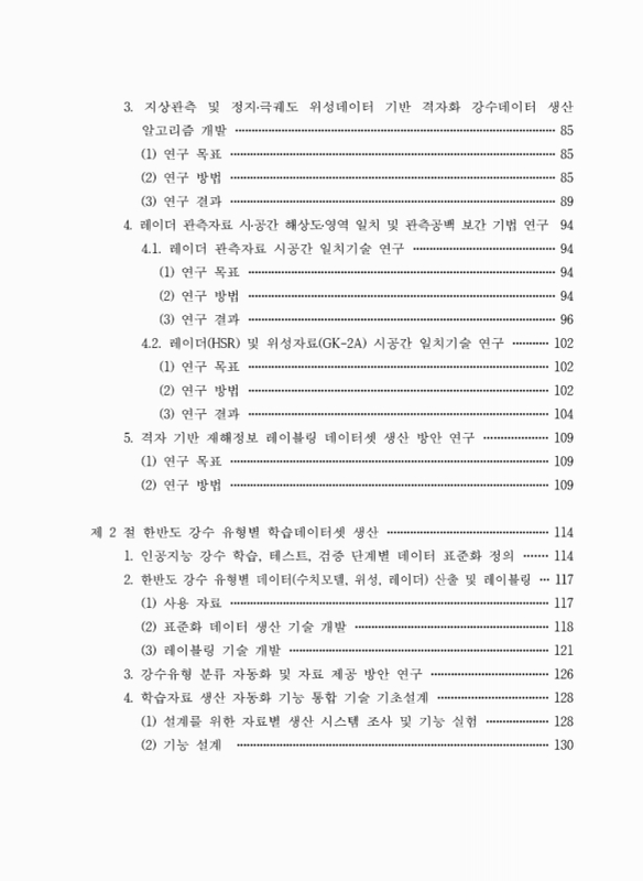
3. 지상관측 및 정지·극궤도 위성데이터 기반 격자화 강수데이터 생산 알고리즘 개발 113
4. 레이더 관측자료 시·공간 해상도·영역 일치 및 관측공백 보간 기법 연구 122
5. 격자 기반 재해정보 레이블링 데이터셋 생산 방안 연구 137
제2절 한반도 강수 유형별 학습데이터셋 생산 142
1. 인공지능 강수 학습, 테스트, 검증 단계별 데이터 표준화 정의 142
2. 한반도 강수 유형별 데이터(수치모델, 위성, 레이더) 산출 및 레이블링 145
3. 강수유형 분류 자동화 및 자료 제공 방안 연구 154
4. 학습자료 생산 자동화 기능 통합 기술 기초설계 156
제3절 3차원 고해상도 자료 생산 기술 연구(제주지역 중심으로) 160
1. 관측자료의 공간해상도 상세화 기술 개발 160
2. 제주지역 3차원 고해상도 실황분석장 생산 방안 연구 167
제4장 3차년도(2024년) 연구결과 177
제1절 정형·비정형 자료 활용 및 융합 기초기술 개발 177
1. 레이더 관측 및 바람장, 수상체 정보 기반 학습데이터셋 개발 및 생산 자동화 177
2. 지상관측 및 정지·극궤도 위성데이터 기반 격자화 강수데이터 생산 자동화 188
3. 레이더 관측공백 보간 기법 개발 198
4. 격자 기반 재해정보 레이블링 데이터셋 생산 220
제2절 한반도 강수 유형별 학습데이터셋 생산 222
1. 한반도 강수 유무 및 유형 분류 과정 자동화 완료 222
2. 위성, 레이더, 수치모델자료 융합 기반 학습자료 표준화 232
3. 학습자료 자동화 통합 및 감시·수동수행 기능 개발 243
제3절 3차원 고해상도 자료 생산 기술 연구(제주지역 중심으로) 249
1. 제주지역 3차원 고해상도 모델기반 분석장 생성 249
2. 제주지역 3차원 고해상도 관측기반 분석장 생성 267
제5장 요약 및 결론 285
1. 정형·비정형 자료 활용 및 융합 기초기술 개발 285
1.1. 정지궤도 기상위성 관측영상 시간(10분 간격), 공간해상도 및 영역 일치 285
1.2. 레이더 관측 및 바람장, 수상체정보 기반 학습데이터셋 개발 및 생산 자동화 286
1.3. 지상관측 및 정지·극궤도 위성데이터 기반 격자화 강수데이터 생산 자동화 287
1.4. 레이더 관측공백 보간 기법 개발 290
1.5. 격자 기반 재해정보 레이블링 데이터셋 생산 292
2. 한반도 강수 유형별 학습데이터셋 생산 293
2.1. 위성, 레이더, 수치모델 자료 학습자료 표준화 294
2.2. 학습자료 자동화 통합 및 감시·수동 수행 기능 295
3. 3차원 고해상도 자료 생산 기술 연구(제주지역 중심으로) 297
3.1. 제주지역 3차원 고해상도 모델기반 분석장 생산 297
3.2. 제주지역 3차원 고해상도 관측기반 분석장 생성 298
참고 문헌 302
부록 1. 주요 성과 304
[뒷표지] 305
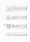
Fig. 2.1.1. Example of alignment of research area for radar HSR, GK-2A, and... 34
Fig. 2.1.2. The data period for train, validation, and application of the model 34
Fig. 2.1.3. Data pair method used in this study 35
Fig. 2.1.4. Structure of Data2Data for this study 36
Fig. 2.1.5. Results of applying GK-2A IR10.5 channel to the generated model 37
Fig. 2.1.6. Scatter plot comparison of each channel between GK-2A and COMS 38
Fig. 2.1.7. Results of model application before and after calibration of the WV channel 40
Fig. 2.1.8. Time series results of applying the temporal resolution enhancement... 40
Fig. 2.1.9. CFAD of WISSDOM wind field u, v, w wind components and... 41
Fig. 2.1.10. Examples of results from performing abrupt change checks and spike checks. 43
Fig. 2.1.11. QC Flag Example(September 6, 2020 22:20 KST) 44
Fig. 2.1.12. (a) Location and interpolation method of AWS(Automatic... 46
Fig. 2.1.13. Four tested precipitation generation algorithm 46
Fig. 2.1.14. Algorithm flowchart of rain data merge 47
Fig. 2.1.15. (a) One-point removal cross-validation error according to case and... 48
Fig. 2.1.16. Example of rain data merge 49
Fig. 2.1.17. Study area(left) and gridded AWS result(right) 51
Fig. 2.1.18. (a) Radar rainfall, (b) AWS rainfall, (c) regression predicted AWS,... 52
Fig. 2.1.19. Results of AWS grid mapping using regression kriging method 53
Fig. 2.1.20. (a) RK AWS, (b) virtual, (c) RK AWS-virtual, (d) map of hit-false-miss,... 54
Fig. 2.1.21. (a) RK AWS, (b) virtual, (c) RK AWS-virtual, (d) map of hit-false-miss,... 54
Fig. 2.1.22. (a) RK AWS, (b) virtual, (c) RK AWS-virtual, (d) map of hit-false-miss,... 55
Fig. 2.1.23. (a) RK AWS, (b) virtual, (c) RK AWS-virtual, (d) map of hit-false-miss,... 55
Fig. 2.2.1. Flowchart of korea's local heavy rain type classification using som algorithm 59
Fig. 2.2.2. Characteristics of spatial distribution by type of local precipitation 60
Fig. 2.2.3. Classification of precipitation types according to cluster analysis. First... 61
Fig. 2.2.4. Precipitation type cluster classification analysis area by variable characteristics 63
Fig. 2.2.5. Dendrogram results of HCA techniques by variable characteristics 64
Fig. 2.2.6. Labeling process flowchart 67
Fig. 2.3.1. Weather categories with exemplary synoptic surface weather map 72
Fig. 2.3.2. (Upper Left) 850 hPa geopotential height(gpm, red contour) and... 73
Fig. 2.3.3. (Upper Left) 850 hPa horizontal gradient of equivalent potential... 74
Fig. 2.3.4. (Upper Left) Difference between the sea surface temperature and 850 hPa... 76
Fig. 2.3.5. (Left) 850 hPa vertical velocity(10⁻¹ ms⁻¹, shading) and horizontal... 77
Fig. 2.3.6. (Left) 850hPa stretching deformation(10⁻⁵ s⁻¹) and (Right) horizontal... 77
Fig. 2.3.7. (Left) 850 hPa gradient of geopotential temperature(10⁻⁵, shading),... 78
Fig. 2.3.8. Location of observation points by observation variables displayed... 81
Fig. 2.3.9. Flow chart of early algorithm for 3-dimensional wind field... 82
Fig. 2.3.10. Radar location and observation radius near Jeju 83
Fig. 2.3.11. Spatial distribution of observations : AWS and ASOS... 85
Fig. 2.3.12. (2023.06.11.0300 UTC) Brightness Temperature of water vapor... 86
Fig. 2.3.13. Domain configuration(9.0, 3.0, 1.0, 0.2km resolution) 88
Fig. 2.3.14. Schematic diagram for constructing gridded PPI 89
Fig. 2.3.15. Generating 10-minute mean data from the KMA's AWS... 91
Fig. 2.3.16. Examples of generating 10-minute average field(wind, temperature,... 91
Fig. 2.3.17. Radial velocity PPI images of CLEANER. 92
Fig. 2.3.18. Validation results of u component of 3-dimensional wind... 94
Fig. 2.3.19. Validation results of v component of 3-dimensional wind... 95
Fig. 3.1.1. Study Area 97
Fig. 3.1.2. Results of applying GK-2A VIS 0.6㎛ channel to the model 98
Fig. 3.1.3. Results of applying GK-2A SW 3.8㎛(day) channel to the model 98
Fig. 3.1.4. Results of applying GK-2A SW 3.8㎛(night) channel to the model 99
Fig. 3.1.5. Results of applying GK-2A WV 6.9㎛ channel to the model 99
Fig. 3.1.6. Results of applying GK-2A IR 10.5㎛ channel to the model 100
Fig. 3.1.7. Results of applying GK-2A IR 12.3㎛ channel to the model 100
Fig. 3.1.8. Results of applying COMS VIS channel to the model. 102
Fig. 3.1.9. Results of applying COMS SWIR(day) channel to the model 103
Fig. 3.1.10. Results of applying COMS SWIR(night) channel to the model 103
Fig. 3.1.11. Results of applying COMS WV channel to the created model 104
Fig. 3.1.12. Results of applying COMS IR01 channel to the created model 104
Fig. 3.1.13. Results of applying COMS IR02 channel to the created model 105
Fig. 3.1.14. Results of improved temporal resolution of COMS IR01 channel 106
Fig. 3.1.15. CFAD image for each R3D radar observation variables 107
Fig. 3.1.16. The flow chart of R3D data pre-processing algorithm 108
Fig. 3.1.17. Normal frequency distribution(black) and cumulative frequency... 109
Fig. 3.1.18. CFAD images before(left) and after(right) applying the R3D... 112
Fig. 3.1.19. Algorithm for grid precipitation using AWS 114
Fig. 3.1.20. WISSDOM area(left) and study area(right) 116
Fig. 3.1.21. ResNet structure utilized in the generator 117
Fig. 3.1.22. Examples of the results of the generation algorithm for rain rate... 117
Fig. 3.1.23. Collocation algorithm flow chart 118
Fig. 3.1.24. Radar-AWS collocation result 119
Fig. 3.1.25. GEO collocation result 119
Fig. 3.1.26. LEO collocation result 119
Fig. 3.1.27. Box-and-whisker plot by evaluation metrics for the test set 120
Fig. 3.1.28. Case analysis(Apr. 26, 2022, 10:00 KST) 121
Fig. 3.1.29. The flowcharts of generation algorithm for gridded... 123
Fig. 3.1.30. Rain merge algorithm flow chart 124
Fig. 3.1.31. R3D reflectivity after spatiotemporal matching(four methods of xemsf) 125
Fig. 3.1.32. Examples of gridded precipitation fields at August 8, 2022 18:00... 126
Fig. 3.1.33. Scatter plot analysis between observation values of AWS and... 127
Fig. 3.1.34. East-Asia domain rain data merging example - 2022.09.0 5. 1340 KST 128
Fig. 3.1.35. Rain merge field scatter plot 129
Fig. 3.1.36. GK-2A(red), radar HSR(blue) data area, and rainfall... 130
Fig. 3.1.37. Case analysis(August 21, 2021, 11:00 KST) 133
Fig. 3.1.38. Stratiform precipitation case analysis(March 04, 2021, 15:00 KST) 134
Fig. 3.1.39. Trend analysis of evaluation metrics for stratiform precipitation cases... 135
Fig. 3.1.40. Convective precipitation case analysis(July 06, 2021, 12:00 KST) 135
Fig. 3.1.41. Trend analysis of evaluation metrics for convective precipitation... 136
Fig. 3.1.42. Grid map with a 0.1° interval in the range of 33~39°N, 125~131°E 139
Fig. 3.1.43. Confirm the positions of grid points with intervals of 0.1° and 0.01° 139
Fig. 3.1.44. Grid points with a spacing of 0.01° included within a 10x10 range... 140
Fig. 3.1.45. 2021.08.22 landslide, disaster(Typhoon) occurrence amount for grid are 141
Fig. 3.2.1. The purpose of each stage in the training dataset. 143
Fig. 3.2.2. Flowchart of labeling process for short-mid-term precipitation types 150
Fig. 3.2.3. Flowchart for short-term precipitation type labeling process 153
Fig. 3.2.4. Automated rainfall type classification system 154
Fig. 3.2.5. Design proposal for a learning dataset generation system 156
Fig. 3.3.1. (a) Algorithm for generating radar-rain gauge merging precipitation field... 161
Fig. 3.3.2. Observed precipitation vs. LOOCV values from (a) AWS, (b) all rain... 162
Fig. 3.3.3.Comparison of observationvalues and LOOCV values before and... 162
Fig. 3.3.4. Flow chart of improved algorithm for 3-dimensional wind field... 163
Fig. 3.3.5. Change of 3-dimensional wind field following surface input data... 165
Fig. 3.3.6. Comparison of u, v, wind speed(WS) with various options. (a)-(c)... 165
Fig. 3.3.7. Comparison of u, v, wind speed(WS) between 3-dimensional... 166
Fig. 3.3.8. Diagram of radar data preprocessing program 168
Fig. 3.3.9. Converted ASOS and AWS data into Little-R format as input for... 169
Fig. 3.3.10. Converted sea-surface data into Little-R format(2023.07.18.0000 UTC)... 170
Fig. 3.3.11. Converted wind profiler data into Little-R format(2023.07.18.0000 UTC) 170
Fig. 3.3.12. Converted rawinsonde data into Little-R format for WRFDA(2023.07.18.0000 UTC) 171
Fig. 3.3.13. Flow chart of the preprocessing program handling... 172
Fig. 3.3.14. Diagram of ASR data preprocessing program 173
Fig. 3.3.15. Diagram of AMV data preprocessing program 173
Fig. 3.3.16. Data assimilation timeline 174
Fig. 3.3.17. (2021.08.10.2200 UTC, Domain 03) (a) Radar reflectivity(dBZ) observation at... 175
Fig. 3.3.18. (2023.11.05.2000UTC) (a), (d) Radar reflectivity(dBZ) observation at 1.5km,... 176
Fig. 4.1.1. STEP test CFAD image before (left) and after (right) adding the... 178
Fig. 4.1.2. Threshold value determination procedure for each test 179
Fig. 4.1.3. Threshold determination process for STEP(CZ) test. 180
Fig. 4.1.4. Comparison of QC flag CAPPI (h=2km) image (a) before and (b)... 182
Fig. 4.1.5. Comparison of QC flag CFAD (a) before and (b) after threshold adjustment 182
Fig. 4.1.6. Reflectivity at 2 km CAPPI image (a) before and (b) after threshold... 183
Fig. 4.1.7. Comparison of reflectivity(CZ) CFAD (a) before and (b) after... 184
Fig. 4.1.8. Comparison of 1 km altitude average reflectivity (a) before and (b)... 184
Fig. 4.1.9. Program flowchart with exception handling applied... 185
Fig. 4.1.10. Example of global properties of R3D preprocessing result file 186
Fig. 4.1.11. Example of log file 187
Fig. 4.1.12. Example of error messages 187
Fig. 4.1.13. AWS-Radar precipitation data production automation algorithm flowchart 189
Fig. 4.1.14. Examples of preferences and options in the 'Config.ini' file 190
Fig. 4.1.15. Examples of each message in the unified log file and error log file 191
Fig. 4.1.16. Algorithm flow chart for LEO collocation 192
Fig. 4.1.17. AWS and radar merging precipitation field comparison test... 193
Fig. 4.1.18. Scatter plot comparison for quantitative validation(period : June... 194
Fig. 4.1.19. Summary of error verification results using bar graphs 195
Fig. 4.1.20. Cumulative Density Function plot for satellite data 196
Fig. 4.1.21. F18 rainfield adjustment example - 2023.08.10. 15:40 KST 197
Fig. 4.1.22. Example of log files for LEO collocation algorithm 197
Fig. 4.1.23. Rain data merge algorithm flow chart 198
Fig. 4.1.24. Example of weight calculation 199
Fig. 4.1.25. Example of ground rain field and satellite rain field, merge rain rain... 201
Fig. 4.1.26. Merge rainfield mean rainrate and GTS mean rainrate - 2023.05.05 203
Fig. 4.1.27. Verification result scatter plot - all case 204
Fig. 4.1.28. Example of log files for rain data merge algorithm 205
Fig. 4.1.29. Correlation analysis between target bands 207
Fig. 4.1.30. MI between target data and all 45 IR band and band difference combinations 208
Fig. 4.1.31. Correlation heatmap by MI values for VIS band generation 209
Fig. 4.1.32. Correlation heatmap by MI values for NIR1.3 band generation 209
Fig. 4.1.33. Correlation heatmap by MI values for NIR1.6 band generation 210
Fig. 4.1.34. Analysis of virtual VIS and NIR band data for the case on... 212
Fig. 4.1.35. Box-and-whisker plot of statistical metrics by band 213
Fig. 4.1.36. Trend analysis of M1, M2, and M3 for the test set by evaluation metrics 214
Fig. 4.1.37. Mean value bar plots for IR model(M1), daytime model, and... 216
Fig. 4.1.38. Estimated results and qualitative comparisons of precipitation in IR... 217
Fig. 4.1.39. Model training area(green), radar HSR data area(blue), overseas... 218
Fig. 4.1.40. Ground radar data and regional generation examples for the daytime... 219
Fig. 4.2.1. Spatial distribution of cape variables for each numerical model 229
Fig. 4.2.2. Standardized production automation system for short-mid-term... 233
Fig. 4.2.3. Standardized production automation system for short-term... 234
Fig. 4.2.4. Area average method(simple average(left), weighted average(right)) 235
Fig. 4.2.5. Examples of grids used according to grid resolution(0.05 degrees(left),... 236
Fig. 4.2.6. Data automation integrated production system schematic diagram 243
Fig. 4.2.7. Schematic diagram of the learning material production monitoring system 246
Fig. 4.2.8. Example of monitoring display on the monitoring webpage 248
Fig. 4.3.1. WRF domain configuration 250
Fig.4.3.2. WRF modeling and assimilation timeline 251
Fig. 4.3.3. O-B BT statistics for GK-2A water vapor channels(Ch 8-10)... 252
Fig. 4.3.4. 7.3㎛ Brightness temperature(K) of GK-2A(Left), WRF... 253
Fig. 4.3.5. 30 minute precipitation of(Left) AWS, (Middle) NoDA, (Right) DA at... 254
Fig. 4.3.6. Water vapor mixing ratio(shading, g kg⁻¹) and wind(vector, ms⁻¹)... 254
Fig. 4.3.7. Cross-section of water vapor mixing ratio(shading, g kg⁻¹) and wind.... 255
Fig. 4.3.8. 30 minute precipitation of (Left) AWS, (Middle) NoDA, (Right) DA at... 256
Fig. 4.3.9. Water vapor mixing ratio(shading, g kg⁻¹) and wind(vector, ms⁻¹) at 850 hPa 257
Fig. 4.3.10. Cross-section of water vapor mixing ratio (shading, g kg⁻¹) and wind... 258
Fig. 4.3.11. 30 minute precipitation of (Left) AWS, (Middle) NoDA, (Right) DA... 259
Fig. 4.3.12. Water vapor mixing ratio(shading, g kg⁻¹) and wind(vector, ms⁻¹) at 850 hPa 260
Fig. 4.3.13. Cross-section of water vapor mixing ratio(shading, g kg⁻¹) and wind vector... 261
Fig. 4.3.14. Scatter plot of GK-2A WV channels BT [K] from(Left) observation... 262
Fig. 4.3.15. NoDA(black), DA_Old(green), and DA_New(blue) MAE and... 264
Fig. 4.3.16. NoDA(black), DA_Old(green), and DA_New(blue) MAE and... 264
Fig. 4.3.17. NoDA(black), DA_Old(green), and DA_New(blue) MAE... 265
Fig. 4.3.18. NoDA(black), DA_Old(green), and DA_New(blue) MAE and... 265
Fig. 4.3.19. MAE improvement rate of DA compared to NoDA(Case 1-5) 266
Fig. 4.3.20. PC improvement rate of DA compared to NoDA(Case 1-5) 266
Fig. 4.3.21. Examples of image files and ASCIIfiles generate with Python code 268
Fig. 4.3.22. Modified quality control code section in the function 'make_QC_flag_other' 268
Fig. 4.3.23. Example if wind filed images before and after quality control 269
Fig. 4.3.24. Examples of temperature field images and nonlinearly... 270
Fig. 4.3.25. Modifications to the code of the 'Nonlinear_AT' function(left)... 270
Fig. 4.3.26. Examples of function forms approximated nonlinearly... 271
Fig. 4.3.27. Examples of temperature fields generated with nonlinear profiles for... 272
Fig. 4.3.28. (a) Radar precipitation, (b) precipitation field merged with existing... 274
Fig. 4.3.29. General settings in the configuration file 274
Fig. 4.3.30. Output option in the configuration file 275
Fig. 4.3.31. Examples of the production images of the ground observation... 276
Fig. 4.3.32. Scatter plot analysis for Case 1 277
Fig. 4.3.33. Examples of the production images of the ground observation... 277
Fig. 4.3.34. Scatter plot analysis for Case 2 278
Fig. 4.3.35. Flow chart of the developed algorithm for 3-dimensional... 279
Fig. 4.3.36. Photographs during installation of CAPPI algorithm in 5th super... 281
Fig. 4.3.37. Photographs during installation of algorithm for 3-dimensional wind... 282
Fig. 4.3.38. (a) Example of log file when algorithm for 3-dimensional... 283
Fig. 4.3.39. Photographs during installation of algorithm for image... 283
Fig. 4.3.40. Plots of 3-dimensional wind field data about 20 : 00 UTC 5 November 2023. 284

※ 출처: 상단의 서지정보에서 확인
※ 원저작물에 적용된 공공누리 유형: 제2유형
| 등록번호 | 청구기호 | 권별정보 | 자료실 | 이용여부 |
|---|---|---|---|---|
| 0003178397 | 551.630285 -25-3 | v.3 | 서울관 인문자연과학자료실(314호) | 이용가능 |
| 0003178398 | 551.630285 -25-3 | v.3 | 서울관 인문자연과학자료실(314호) | 이용가능 |
*표시는 필수 입력사항입니다.
| 전화번호 |
|---|
| 기사명 | 저자명 | 페이지 | 원문 | 기사목차 |
|---|
| 번호 | 발행일자 | 권호명 | 제본정보 | 자료실 | 원문 | 신청 페이지 |
|---|
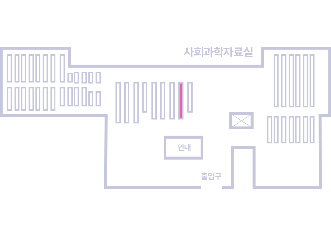
도서위치안내: 인문자연과학자료실(314호) / 서가번호: 33
우편복사 목록담기를 완료하였습니다.
*표시는 필수 입력사항입니다.
저장 되었습니다.